pySpecData: compact spectral data processing!

pySpecData allows you to deal with multi-dimensional spectroscopy data in an object-oriented fashion. This has many benefits, which you can read about below, or check out in the example gallery (menu to the left).

Please note this package is heavily utilized by two other packages that our lab manages on github:

• Classes for communicating with instruments.

  • Controls USB instrumentation like oscilloscopes and power meters connected via a USB/GPIB converter.

  • Includes our Custom SpinCore NMR extension

  • (Note that the previous two used be separate repositories – they have been combined to improve maintenance).

• Processing scripts library that does things like:

  • Automatically process ODNP data.

  • Correlation alignment.

  • Phasing of echo-like NMR data.

  • Quantitative ESR calculation.

  • Aligning ESR spectra for maximum overlap.

  • …*etc*…

The Basics

Our goal is that after you put in a little effort to learn the new way of manipulating data with pySpecData, you can then make the code for processing spectral data that is shorter and that can be written and read in a shorter amount of time (vs using standard numpy). PySpecData automatically handles the following issues, without any additional code:

• relabeling axes after a Fourier transformation

• propagation of errors

• adding units to plots

• calculating analytical Jacobians used during least-squares fitting

To enable this, you work with a pySpecData nddata object (which includes information about dimension names, axis values, errors, and the units) rather than working directly with traditional numpy ndarray objects. (pySpecData is built on top of numpy.)

If you have ever worked with arrays in Matlab or Python before, you are familiar with the additional code needed to convert between index numbers and axis values. Using the funny notation of pySpecData, you can do this automatically.

For example, say you have loaded an nddata object called d and you want to take the time-domain data and:

1. Fourier transform,

2. Select out the central 20 kHz in the frequency domain, and finally

3. Inverse Fourier transform

… all while preserving the correct axes throughout. That looks like this:

>>> d.ft('t2', shift=True)
>>> d = d['t2':(-10e3,10e-3)]
>>> d.ift('t2')

Note that most pySpecData methods operate in-place on the data; it modifies the data inside the nddata, rather than making a new copy. This is because we assume that we are progressively optimizing/filtering our spectral data with each new line of code. This allows us to quickly work through many operations (like the ft here) without keeping many copies of a large dataset and with less typing for each operation. (If you ever truly want to create a copy a dataset, just attach a .C)

Note that

>>> plot(d)

Quickly generates a publication-quality plot; it automatically plots the data on the correct axes and includes the units and the name of dimension (t2 in this example) and its units along the x axis.

Because the axes are tracked transparently, pySpecData is easy to integrate into graphical interfaces. Our FLInst package makes heavy use of this feature to acquire data in real time, as shown below.

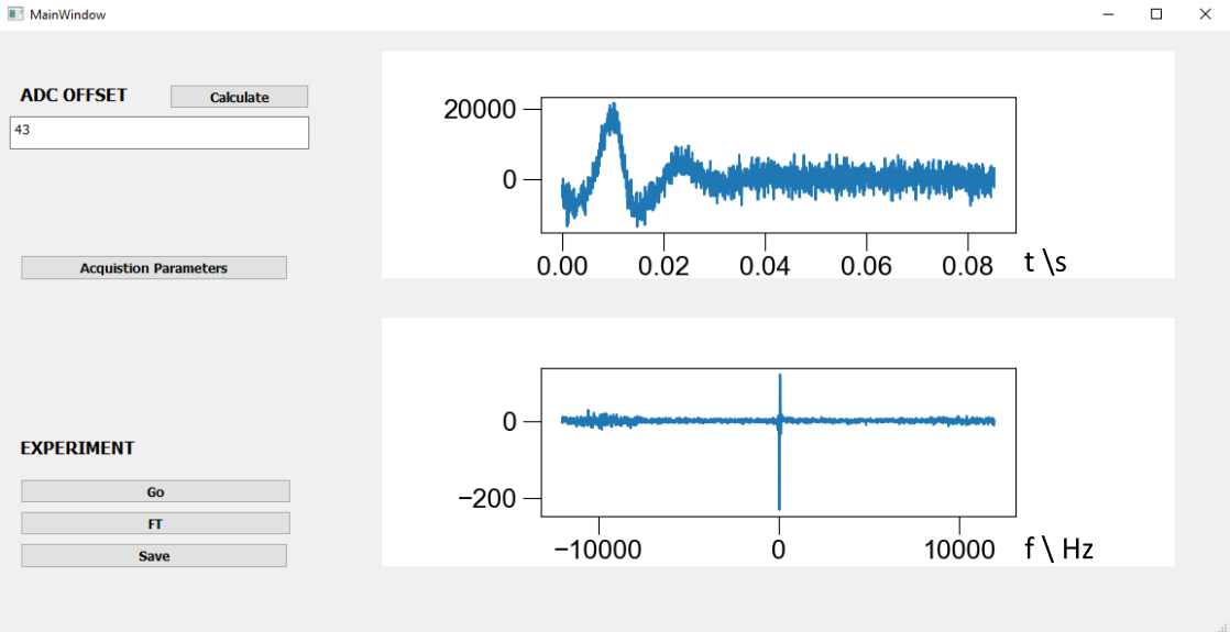
A simple GUI window can be used to acquire a spin echo and immediately Fourier transform the result.

How do I generate an nddata object?

We primarily work in magnetic resonance, so have written wrappers for a few different types of NMR (nuclear magnetic resonance) and ESR (electron spin resonance) file formats. You can use the pyspecdata.find_file() function to automatically load them as nddata.

Additionally, we have written several classes that allow you to read nddata objects directly from e.g. an oscilloscope. These are available in separate repositories on github.

Finally, you can easily build nddata from standard arrays, as discussed in the section about nddata objects.

What can I do with nddata objects?

To understand how to manipulate nddata objects, head over to the section about nddata objects.

You are strongly encouraged to check out the example gallery (menu to the left) both for this repo, and for the companion processing scripts library.

Contents:

There are many other features of pySpecData that govern the interaction of ndata objects with plots and, e.g. that allow you to generate a nice PDF laboratory notebook showing every step of your data processing. These and further details are covered in the various sections of the documentation:

• ND-Data
  • Multidimensional data
  • Building an nddata from numpy arrays
  • Dimension labels
  • Item selection and slicing
  • Error propagation
  • Methods for Manipulating Data
  • Basic Examples
  • Methods by Sub-Topic
• the lmfitdata class
  • lmfitdata
• List of Modules and Sub-Packages
  • core
  • figlist
  • general_functions
  • datadir
  • load_files
  • fornotebook
  • latexscripts
  • ipy
  • ndshape
  • units
• LaTeX Notebook Functionality
  • Setting up the notebook
  • Running the notebook
  • How it works
• The Figure List
• Units
  • units

Example Gallery

• PySpecData Examples
  • DCCT
  • ESR
  • UV
  • XX Individual Functions XX

Instrumentation use cases

PySpecData interfaces with a variety of laboratory hardware. The diagram below summarizes how the resonator, RF transceiver and control computer are connected. This setup comes from our lab and represents just one example of how pySpecData can be used alongside instrumentation.

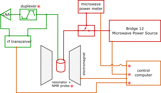
Modular EPR/NMR instrument layout.

Experiment pulse programs are uploaded to a SpinCore PulseBlaster as shown below.

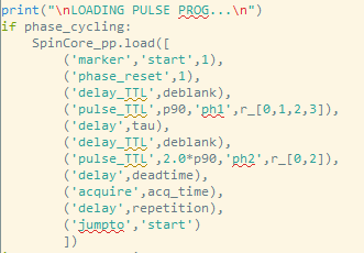
Loading a PulseBlaster program with phase cycling.

A close-up of the PCIe board used for TTL control is shown here.

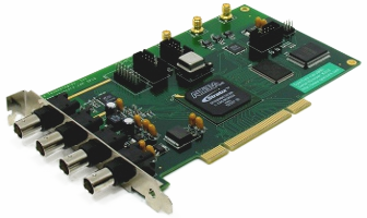
SpinCore PulseBlaster board used for TTL control.

One question is – how do we take information from this board as one unit/object and manipulate it seamlessly?

As other example, what if you want to take a basic instrument, like an oscilloscope, and use it to do something mildly more complicated, like measure the response of an NMR probe? We can do this by isolating the envelope of the probe’s ring-down and fitting it to an exponential decay. Even though the signal looks like this:

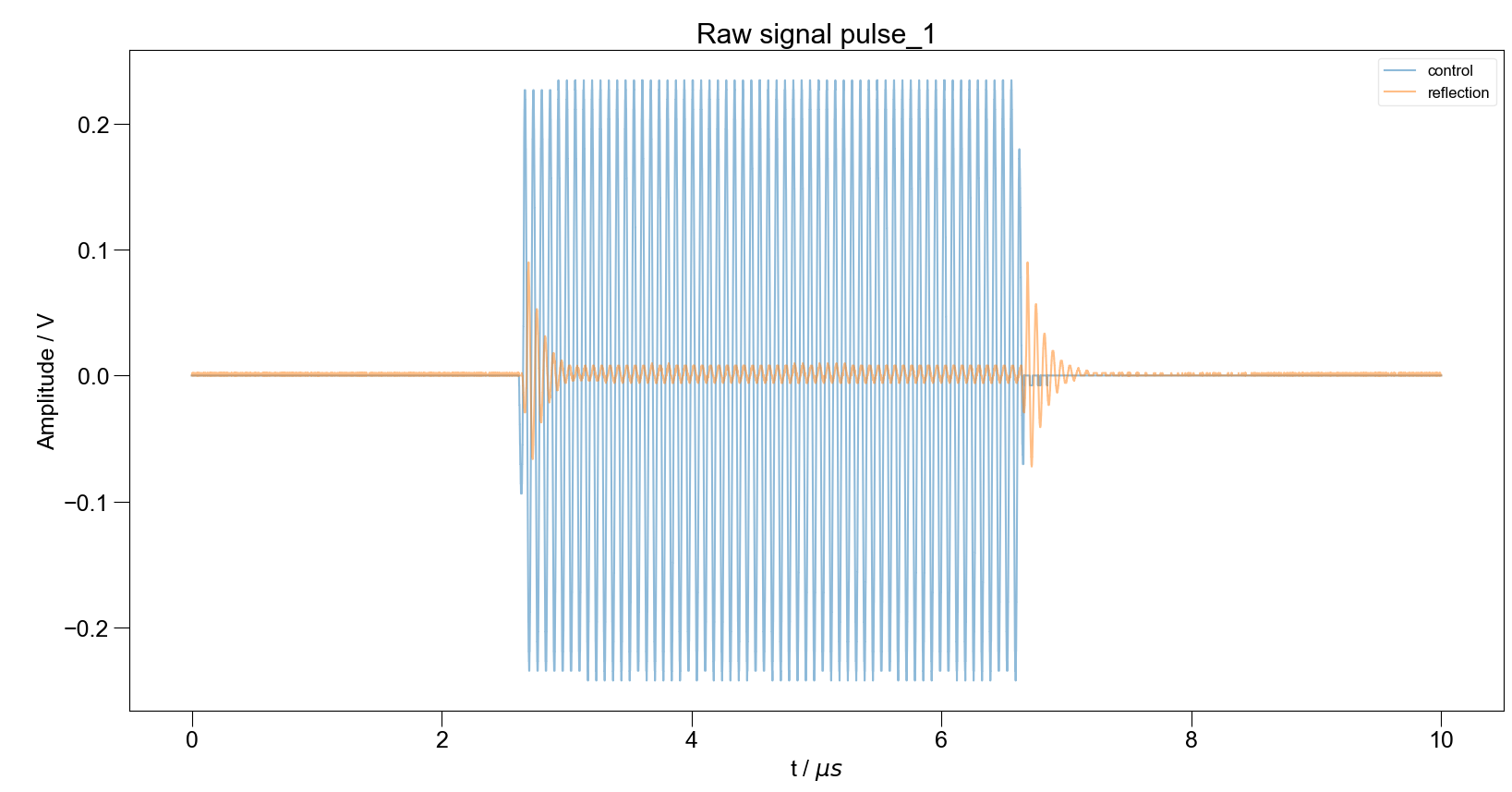
Raw pulse and reflection used for the measurement.

To interpret it meaningfully, we want to convert to analytic signal, as we show below. The key is that to perform these types of manipulations:

• We want to easily move back and forth between the frequency and time domain, while having axes with real units.

• The computer likes to refer to the index/position of a datapoint in a dataset (think frequency spectrum), but we want to be able to use natural/intuitive notation for things like frequency selection and filtration.

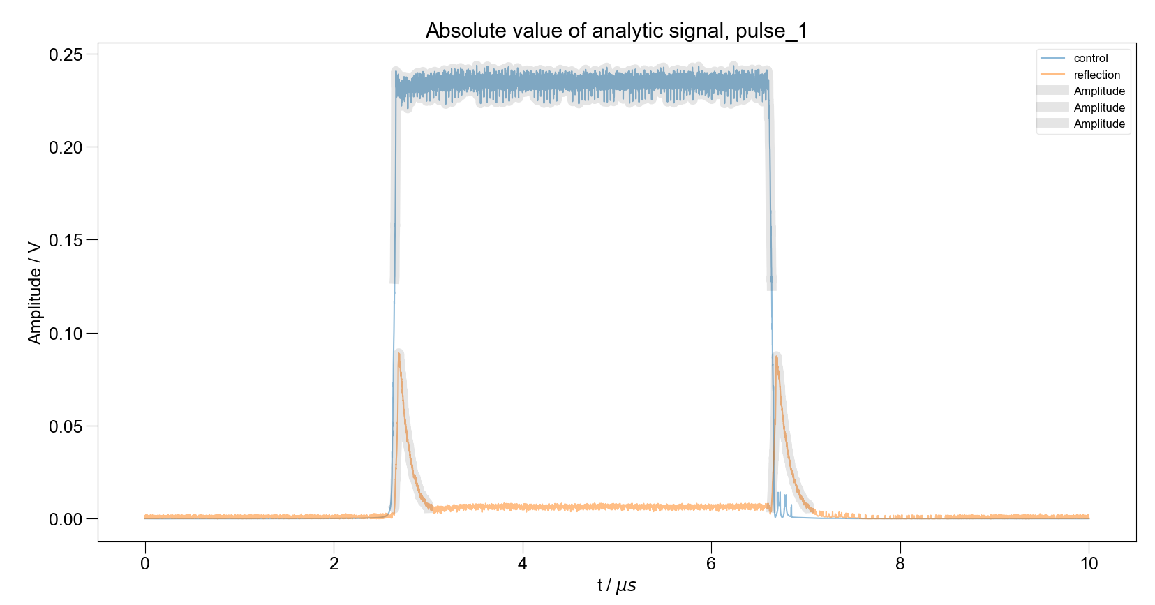
Analytic-signal envelope of the reflection. (This is the magnitude of the analytic signal, while the phase gives us information about phase/frequency.)

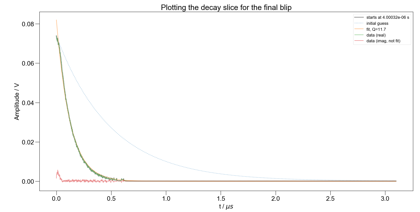
Exponential fit to the decay slice tells us about the \(Q\)-factor (while the phase tells us about resonance offset).

For more examples of specific implementations, see our processing scripts library.

Indices and tables

• Index

• Module Index

• Search Page