ND-Data
(This is an introduction. For detailed info, see API documentation.)
The nddata class is built on top of numpy. Numpy allows you to create multi-dimensional arrays of data.
Conceptually, an nddata instance acts as a container that holds the raw
array along with its descriptive metadata. A schematic view of this
structure appears in nddata-container-fig inside the
API documentation for pyspecdata.nddata.
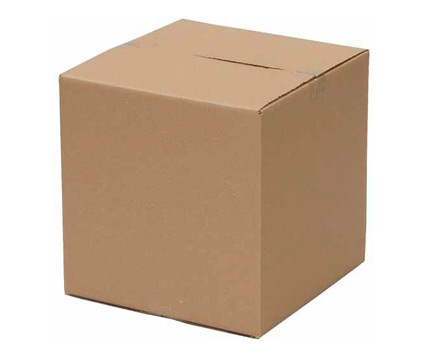
A simple container metaphor for an nddata object.

Axes, units and error arrays are stored alongside the data itself.
Multidimensional data
The nddata class labels the dimensions (with a short text identifier) and allows you to associate axes, units, and errors with the data. These attributes are correctly transformed when you perform arithmetic operations or Fourier transforms, and are used to automatically format plots.
Very importantly, most pyspecdata functions are designed to operate on the data in place, meaning that rather than doing something like:
>>> data = data.mean() # numpy
you simply do:
>>> data.mean('axisname')
and data is modified from here out.
We do this because we are typically processing multidimensional datasets that consist of many points,
and we subject them to a series of steps to process them.
We don’t want to use up memory with lots of copies of the data.
Also, this allows us to string together several operation, e.g.:
>>> data.ft('axis1').sum('axis2').mean('axis3')
So, while this general setup is different than the standard numpy setup, etc., it should lead to you writing more efficient code, with less variables to keep track of, and generally also leads to far more compact code, and you should probably not try to bypass it by creating copies of your data.
The next figure contrasts a plain two-dimensional numpy array with the richer nddata representation.
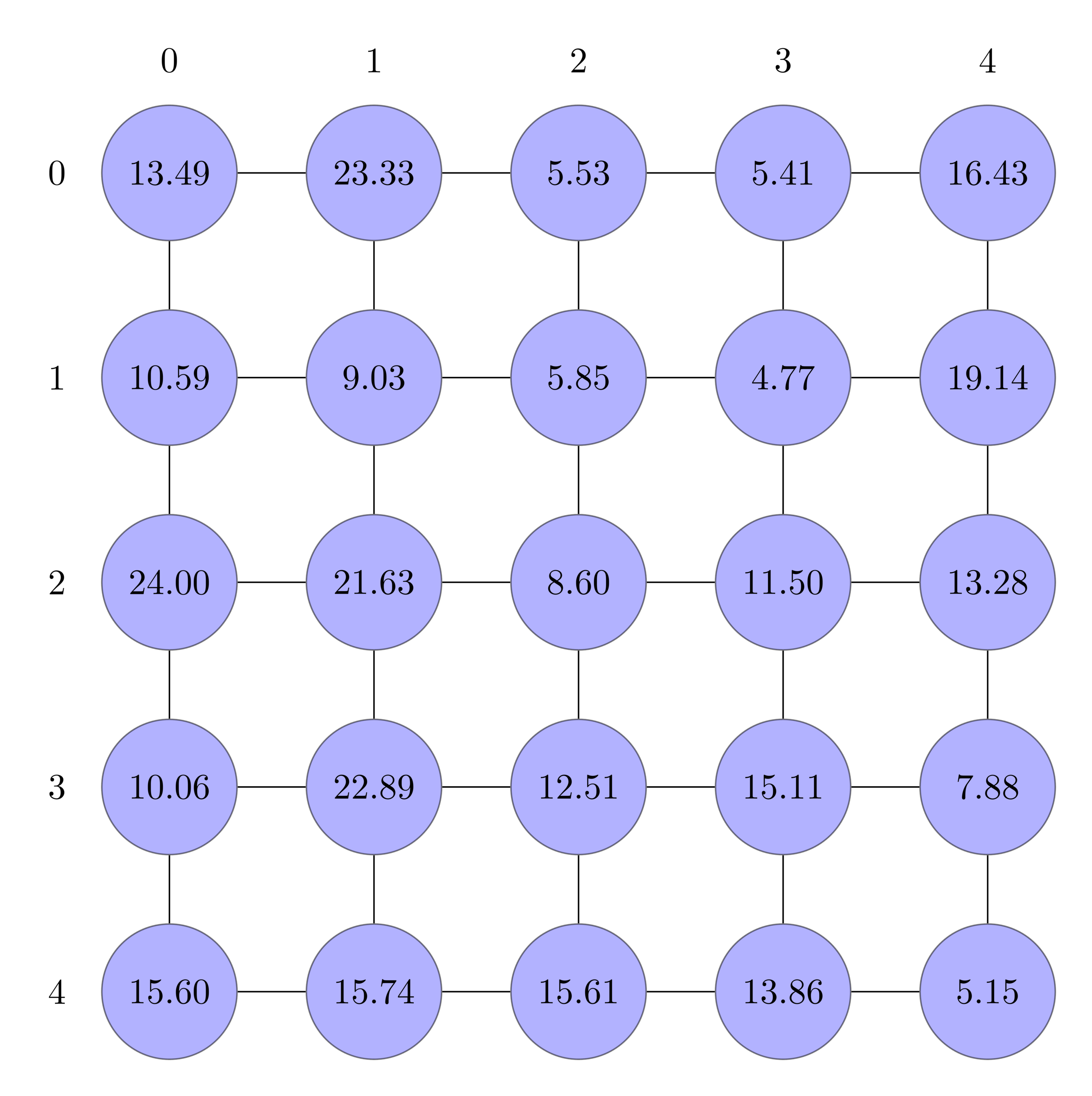
A traditional 2D numpy array for comparison.
The nddata object keeps track of dimension names, coordinate axes and their uncertainties, making operations and plotting far easier.
In rare circumstances, you need to create a copy of your data (I think there is only one case where this is true: when you need to process the same data in parallel in two different ways to generate two results, and then perform math that uses both results). For these cases, you can use an easy shortcut for the copy method: C (as in data.C).
Note that, if all else fails,
you can always use numpy directly:
The `data` attribute of an nddata object is just a standard numpy array.
For example, if you have an nddata object called mydata,
then mydata.data is just a standard numpy array.
But, note that – in most cases – it should be more beneficial if you don’t
directly access the data attribute.
Below, we outline how you can use dimension labels to make code more legible and make many common tasks easier. Then, we note how slicing operations are different (and easier) for nddata than for standard numpy arrays. Finally, we outline several classes of methods by sub-topic.
Building an nddata from numpy arrays
You can build nddata objects manually, and we do this a bit in our examples (in order to provide a simple example). However, in practice, you should first ask yourself whether there is already a means for loading your data from a source file or an instrument automatically. If not, it’s still relatively simple to construct your own nddata.
For example, let’s consider a case where we have x and y data
>>> from numpy import *
>>> x = r_[0, 1, 2, 3, 4]
>>> y = r_[0, 0.1, 0.2, 0.3, 0.4]
To transform this into an ndata, we assign y as the data, and label it with x as the axis label.
>>> d = nddata(y,'x').labels('x',x)
The first function nddata(y,'x') creates an instance of nddata; to do this,
we need to give our dimensions names – here we name the single dimension
‘x’.
We then attach an axis label with .labels(‘x’,x)
Now, for example, we’re ready to plot with axis labels or to Fourier transform. However, the true strength of pySpecData lies in how it treats multi-dimensional data.
Note
Please note that the xarray package is another package that deals with multidimensional data, and it does have some of the benefits listed here, but follows a distinctly different philosophy. Here, we place a strong an emphasis on benefits that can be derived from object-oriented programming.
For example, we emphasize effort-free error propagation and Fourier transformation, as well as a compact and meaningful slicing notation.
Dimension labels
All dimension labels can have a display name (used for printing and plotting) and one or more short names (used for writing code).
You don’t need to keep track of the order of dimensions or align dimensions during multiplication. When you do arithmetic with two arrays, pyspecdata will first reshape the arrays so that dimensions with the same names are aligned with each other. Furthermore, during an arithmetic operation, if a dimension is present in one array but not the other, pyspecdata will simply tile the smaller array along the missing dimension(s).
To see how this works, compare the results of
>>> a = nddata(r_[0:4],'a')
>>> b = nddata(r_[0:4],'a')
>>> a*b
[0, 1, 4, 9]
                +/-None
        dimlabels=['a']
        axes={`a':[0, 1, 2, 3]
                        +/-None}
which are arrays of data organized along the same dimension, and
>>> a = nddata(r_[0:4],'a')
>>> b = nddata(r_[0:4],'b')
>>> print a*b
[[0, 0, 0, 0]
 [0, 1, 2, 3]
 [0, 2, 4, 6]
 [0, 3, 6, 9]]
                +/-None
        dimlabels=['a', 'b']
        axes={`a':[0, 1, 2, 3]
                        +/-None,
                `b':[0, 1, 2, 3]
                        +/-None}
which are arrays of data organized along two different dimensions. The figure below shows how independent axes are expanded during such operations.
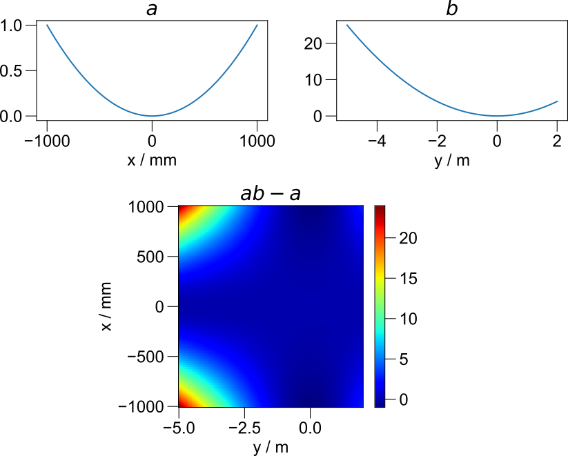
Smart dimensionality when combining independent axes.
You can refer to a time dimension, such as t1, t_1, t_direct, etc. as f1, f_1, etc. in order to retrieve the Fourier transform. You can set the pairs …
Item selection and slicing
Pyspecdata offers several different synataxes for item selection and slicing. These fall into two main categories:
numbered indexing and slicing. These will be familiar to most users of python, but require the addition of the dimension name.
and
axis-coordinate-based. These use the natural axis coordinates. For example, you can specify a range of frequencies, etc., directly, and with a very compact syntax.
Axis-coordinate-based Indexing
To pull a single point along a particular dimension, you can just use the value of the axis. The point nearest to the axis will be returned.
>>> d['t2':1.1]
Will return the point (or slice of data) where the t2 axis is closest to 1.1 s.
Ranges that use Axis Coordinates
You can specify an inclusive range of numbers along an axis. For example, to select from 0 to 100 μs along t2, you use:
>>> d['t2':(0,100e-6)]
Either value in parentheses can be None, in which case, all values to the end of the axis will be selected.
Numbered Indexing and Slicing
You can still use standard index-based references or slices: you do this by placing a comma after your dimension name, rather than a colon:
>>> d['t2',5] # select index 5 (6th element)
>>> d['t2',5::-2] # select from index 5 up to 2 elements before the end
Selection Based on Logic
You can use functions that return logical values to select
>>> d[lambda x: abs(x-2)<5]
returns all data values that are less 5 away from 2 (values from -3 to 8).
>>> d['t2',lambda x: abs(x-2)<5]
When this is done, nddata will check to see if slices along any dimension are uniformly missing. If they are, the dataset will be trimmed to remove them.
When the deselected data are scattered throughout, a mask is used instead.
The .contiguous( method
The contiguous() method deserves special mention,
since it can be used to generate a series of ranges based on logic.
For example, peak selection frequently uses the
contiguous() method.
Selecting and manipulating the axis coordinates
Sometimes, rather than manipulating the data, you want to manipulate the axis coordinates. This is achieve by using square brackets with only the name of the relevant dimension.
For example:
>>> print(data['t2'][1] - data['t2'][0])
tells you the spacing between the first two points along the \(t_2\) axis.
Also,
>>> data['t2'] += 2e-3
adds an offset of 3 ms (assuming your units are seconds) to the \(t_2\) axis.
Error propagation
Todo
this works very well, but show an example here.
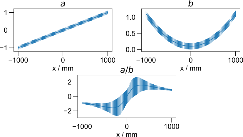
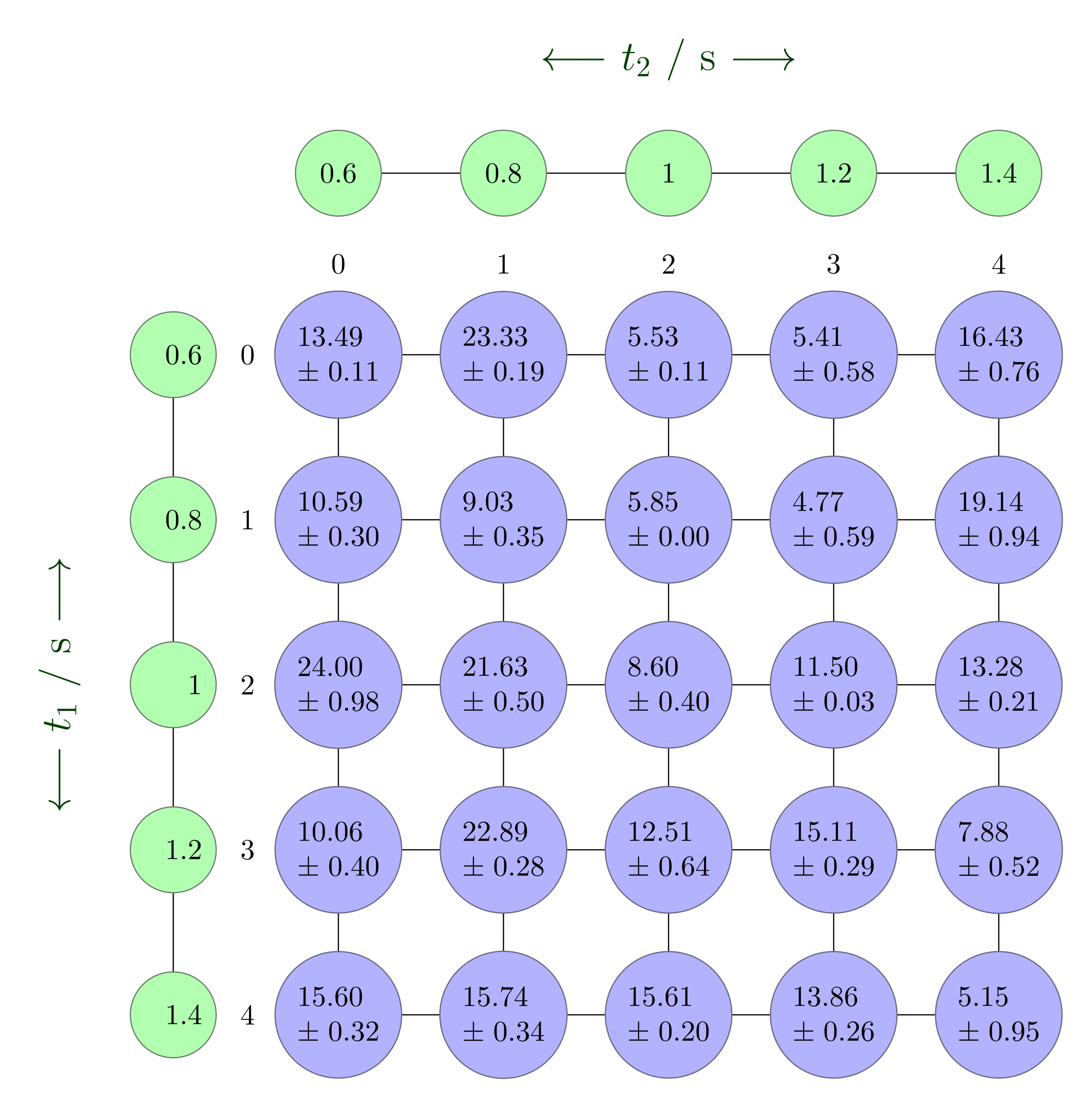
Automatic propagation of errors during arithmetic operations.
Methods for Manipulating Data
It’s important to note that, in contrast to standard numpy,
nddata routines are designed to be called as methods,
rather than independent functions.
Also, these methods modify the data in-place rather than returning a copy.
For example, after executing d.ft('t2') the object d now contains the
Fourier-transformed data. The axes are relabeled automatically, as shown
below.
Automatic relabeling of the frequency axis.
There is no need to assign the result to a new variable.
Alternatively, the property C offers easy access to a copy:
a = d.C.ft('t2') leaves d alone, and returns the FT as a new object
called a.
This encourages a style where methods are chained together, e.g. d.ft('t2').mean('t1').
In order to encourage this style, we provide the method run(), which allows you to run a standard numpy function on the data:
d.run(abs) will take the absolute value of the data in-place, while
d.run(std,'t2') will run a standard deviation along the ‘t2’ axis
(this removes the ‘t2’ dimension once you’re done, since it would have a length of only 1 – run_nopop() would not remove the dimension).
For a full list of methods, see the API documentation: nddata.
Basic Examples
Todo
Give good examples/plots here
Apply a filter (fromaxis).
Slicing.
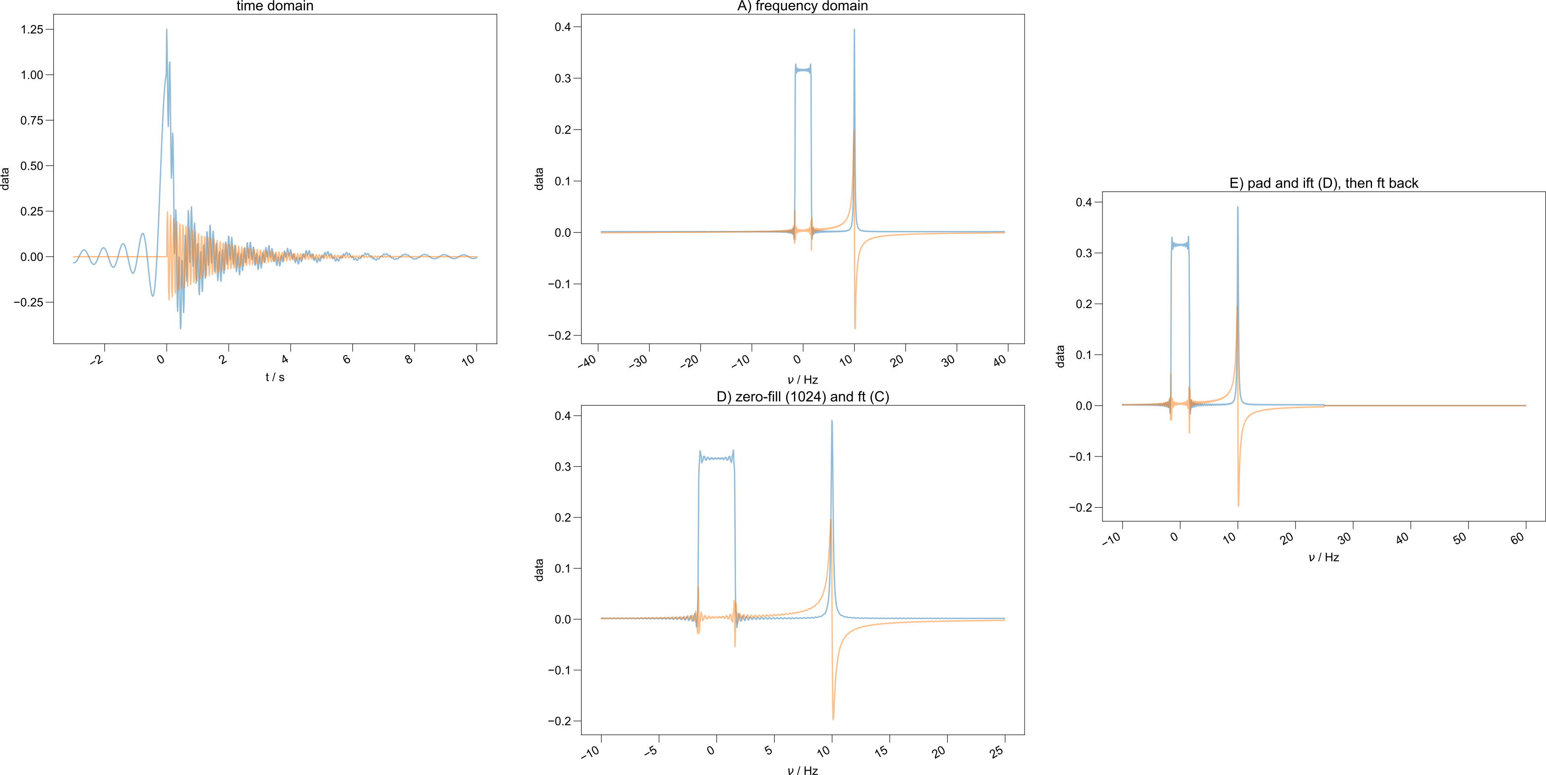
Aliasing of FT.
See ft_new_startpoint() for example
plots demonstrating aliasing and time-origin correction.
Methods by Sub-Topic
Todo
We are in the process of organizing most methods into categories. For now, we encourage you to look through the gallery examples and to click on or search different methods.
A selection of the methods noted below are broken down by sub-topic.