N-dimensional Data (nddata)
By Topic
Full list of nddata methods
- class pyspecdata.nddata(*args, **kwargs)
This is the detailed API reference. For an introduction on how to use ND-Data, see the Main ND-Data Documentation.
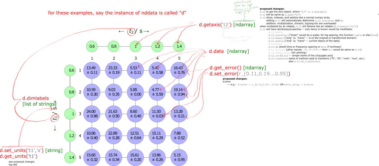
This annotated diagram highlights the attributes stored within an
nddatainstance and how they can be accessed.¶- property C
shortcut for copy
btw, what we are doing is analogous to a ruby function with functioname!() modify result, and we can use the “out” keyword in numpy.
- ..todo::
(new idea) This should just set a flag that says “Do not allow this data to be substituted in place,” so that if something goes to edit the data in place, it instead first makes a copy.
also here, see Definition of shallow and deep copy
(older idea) We should offer “N”, which generates something like a copy, but which is sets the equivalent of “nopop”. For example, currently, you need to do something like
d.C.argmax('t2'), which is very inefficient, since it copies the whole np.array. So, instead, we should dod.N.argmax('t2'), which tells argmax and all other functions not to overwrite “self” but to return a new object. This would cause things like “run_nopop” to become obsolete.
- add_noise(intensity)
Add Gaussian (box-muller) noise to the data.
- Parameters:
intensity (double OR function) – If a double, gives the standard deviation of the noise. If a function, used to calculate the standard deviation of the noise from the data: e.g.
lambda x: max(abs(x))/10.
- aligndata(arg)
This is a fundamental method used by all of the arithmetic operations. It uses the dimension labels of self (the current instance) and arg (an nddata passed to this method) to generate two corresponding output nddatas that I refer to here, respectively, as A and B. A and B have dimensions that are “aligned” – that is, they are identical except for singleton dimensions (note that numpy automatically tiles singleton dimensions). Regardless of how the dimensions of self.data and arg.data (the underlying numpy data) were ordered, A.data and B.data are now ordered identically, where dimensions with the same label (.dimlabel) correspond to the same numpy index. This allows you do do math.
Note that, currently, both A and B are given a full set of axis labels, even for singleton dimensions. This is because we’re assuming you’re going to do math with them, and that the singleton dimensions will be expanded.
- Parameters:
arg (nddata or np.ndarray) – The nddata that you want to align to self. If arg is an np.ndarray, it will try to match dimensions to self based on the length of the dimension. Note: currently there is an issue where this will only really work for 1D data, since it first makes an nddata instance based on arg, which apparently collapses multi-D data to 1D data.
- Returns:
A (nddata) – realigned version of self
B (nddata) – realigned version of arg (the argument)
- along(dimname, rename_redundant=None)
Specifies the dimension for the next matrix multiplication (represents the rows/columns).
- Parameters:
dimname (str) –
The next time matrix multiplication is called, ‘dimname’ will be summed over. That is, dimname will become the columns position if this is the first matrix.
If along is not called for the second matrix, dimname will also take the position of rows for that matrix!
rename_redundant (tuple of str or (default) None) –
If you are multiplying two different matrices, then it is only sensible that before the multiplication, you should identify the dimension representing the row space of the right matrix and the column space of the left matrix with different names.
However sometimes (e.g. constructing projection matrices) you may want to start with two matrices where both the row space of the right matrix and the column space of the left have the same name. If so, you will want to rename the column space of the resulting matrix – then you pass
rename_redundant=('orig name','new name')
- property angle
Return the angle component of the data.
This has error, which is calculated even if there is no error in the original data – in the latter case, a uniform error of 1 is assumed. (This is desirable since phase is a tricky beast!)
- argmax(*axes, **kwargs)
If .argmax(‘dimname’) find the max along a particular dimension, and get rid of that dimension, replacing it with the coordinate where the max value is found.
If .argmax(): return a dictionary giving the coordinates of the overall maximum point.
- Parameters:
raw_index (bool) – Return the raw (np.ndarray) numerical index, rather than the corresponding axis value. Note that the result returned is still, however, an nddata (rather than numpy np.ndarray) object.
- argmin(*axes, **kwargs)
If .argmin(‘dimname’) find the min along a particular dimension, and get rid of that dimension, replacing it with the coordinate where the min value is found.
If .argmin(): return a dictionary giving the coordinates of the overall minimum point.
- Parameters:
raw_index (bool) – Return the raw (np.ndarray) numerical index, rather than the corresponding axis value. Note that the result returned is still, however, an nddata (rather than numpy np.ndarray) object.
- axis(axisname)
returns a 1-D axis for further manipulation
- axlen(axis)
return the size (length) of an axis, by name
- Parameters:
axis (str) – name of the axis whos length you are interested in
- axn(axis)
Return the index number for the axis with the name “axis”
This is used by many other methods. As a simple example, self.:func:axlen`(axis) (the axis length) returns ``np.shape(self.data)[self.axn(axis)]`
- Parameters:
axis (str) – name of the axis
- cdf(normalized=True, max_bins=500)
calculate the Cumulative Distribution Function for the data along axis_name
only for 1D data right now
- Returns:
A new nddata object with an axis labeled values, and data
corresponding to the CDF.
- chunk(axisin, *otherargs)
“Chunking” is defined here to be the opposite of taking a direct product, increasing the number of dimensions by the inverse of the process by which taking a direct product decreases the number of dimensions. This function chunks axisin into multiple new axes arguments.:
axesout – gives the names of the output axes shapesout – optional – if not given, it assumes equal length – if given, one of the values can be -1, which is assumed length
When there are axes, it assumes that the axes of the new dimensions are nested – e.g., it will chunk a dimension with axis: [1,2,3,4,5,6,7,8,9,10] into dimensions with axes: [0,1,2,3,4], [1,6]
- ..todo::
Deal with this efficiently when we move to new-style axes
- chunk_auto(axis_name, which_field=None, dimname=None)
assuming that axis “axis_name” is currently labeled with a structured np.array, choose one field (“which_field”) of that structured np.array to generate a new dimension Note that for now, by definition, no error is allowed on the axes. However, once I upgrade to using structured arrays to handle axis and data errors, I will want to deal with that appropriately here.
- contiguous(lambdafunc, axis=None, return_idx=False)
Return contiguous blocks that satisfy the condition given by lambdafunc
this function returns the start and stop positions along the axis for the contiguous blocks for which lambdafunc returns true Currently only supported for 1D data
Note
- adapted from
stackexchange post http://stackoverflow.com/questions/4494404/find-large-number-of-consecutive-values-fulfilling-condition-in-a-numpy-array
- Parameters:
lambdafunc (types.FunctionType) – If only one argument (lambdafunc) is given, then lambdafunc is a function that accepts a copy of the current nddata object (self) as the argument. If two arguments are given, the second is axis, and lambdafunc has two arguments, self and the value of axis.
axis ({None,str}) – the name of the axis along which you want to find contiguous blocks
- Returns:
retval – An \(N\times 2\) matrix, where the \(N\) rows correspond to pairs of axis label that give ranges over which lambdafunc evaluates to True. These are ordered according to descending range width.
- Return type:
np.ndarray
Examples
sum_for_contiguous = abs(forplot).mean('t1')
fl.next("test contiguous")
forplot = sum_for_contiguous.copy().set_error(None)
fl.plot(forplot,alpha = 0.25,linewidth = 3)
print("this is what the max looks like",0.5*sum_for_contiguous.\
        set_error(None).runcopy(max,'t2'))
print(sum_for_contiguous > 0.5*sum_for_contiguous.\
        runcopy(max,'t2'))
retval = sum_for_contiguous.contiguous(quarter_of_max,'t2')
print("contiguous range / 1e6:",retval/1e6)
for j in range(retval.shape[0]):
    a,b = retval[j,:]
    fl.plot(forplot['t2':(a,b)])
- contour(labels=True, **kwargs)
Contour plot – kwargs are passed to the matplotlib contour function.
See docstring of figlist_var.image() for an example
- labels
Whether or not the levels should be labeled. Defaults to True
- Type:
boolean
- convolve(axisname, filterwidth, convfunc='gaussian', enforce_causality=True)
Perform a convolution.
- Parameters:
axisname (str) – apply the convolution along axisname
filterwidth (double) – width of the convolution function (the units of this value are specified in the same domain as that in which the data exists when you call this function on said data)
convfunc (function) – A function that takes two arguments – the first are the axis coordinates and the second is filterwidth (see filterwidth). Default is a normalized Gaussian of FWHM (\(\lambda\)) filterwidth For example if you want a complex Lorentzian with filterwidth controlled by the rate \(R\), i.e. \(\frac{-1}{-i 2 \pi f - R}\) then
convfunc = lambda f,R: -1./(-1j*2*pi*f-R)enforce_causality (boolean (default true)) –
make sure that the ift of the filter doesn’t get aliased to high time values.
”Causal” data here means data derived as the FT of time-domain data that starts at time zero – like an FID – for which real and abs parts are Hermite transform pairs.
enforce_causality should be True for frequency-domain data whose corresponding time-domain data has a startpoint at or near zero, with no negative time values – like data derived from the FT of an IFT. In contrast, for example, if you have frequency-domain data that is entirely real (like a power spectral density) then you want to set enforce_causality to False.
It is ignored if you call a convolution on time-domain data.
- copy(data=True)
Return a full copy of this instance.
Because methods typically change the data in place, you might want to use this frequently.
- Parameters:
data (boolean) –
Default to True. False doesn’t copy the data – this is for internal use, e.g. when you want to copy all the metadata and perform a calculation on the data.
The code for this also provides the definitive list of the nddata metadata.
- copy_props(other)
Copy all properties (see
get_prop()) from another nddata object – note that these include properties pertaining the the FT status of various dimensions.
- cov_mat(along_dim)
calculate covariance matrix for a 2D experiment
- Parameters:
along_dim (str) – the “observations” dimension of the data set (as opposed to the variable)
- cropped_log(subplot_axes=None, magnitude=4)
For the purposes of plotting, this generates a copy where I take the log, spanning “magnitude” orders of magnitude. This is designed to be called as abs(instance).cropped_log(), so it doesn’t make a copy
- div_units(*args, **kwargs)
divide units of the data (or axis) by the units that are given, and return the multiplier as a number.
In other words, if you pass “a” and the units of your data are in “b”, then this returns x, such that (x a)/(b) = 1.
If the result is not dimensionless, an error will be generated.
e.g. call as d.div_units(“axisname”,”s”) to divide the axis units by seconds.
or d.div_units(“s”) to divide the data units by seconds.
e.g. to convert a variable from seconds to the units of axisname, do var_s/d.div_units(“axisname”,”s”)
e.g. to convert axisname to μs, do d[“axisname”] *= d.div_units(“axisname”,”μs”)
- dot(arg)
This will perform a dot product or a matrix multiplication. If one dimension in
argmatches that inself, it will dot along that dimension (take a matrix multiplication where that dimension represents the columns ofselfand the rows ofarg)Note that if you have your dimensions named “rows” and “columns”, this will be very confusing, but if you have your dimensions named in terms of the vector basis they are defined/live in, this makes sense.
If there are zero or no matching dimensions, then use
along()to specify the dimensions for matrix multiplication / dot product.
- eval_poly(c, axis, inplace=False, npts=None)
Take c output (array of polynomial coefficents in ascending order) from
polyfit(), and apply it along axis axis- Parameters:
c (ndarray) – polynomial coefficients in ascending polynomial order
- extend(axis, extent, fill_with=0, tolerance=1e-05)
Extend the (domain of the) dataset and fill with a pre-set value.
The coordinates associated with axis must be uniformly ascending with spacing \(dx\). The function will extend self by adding a point every \(dx\) until the axis includes the point extent. Fill the newly created datapoints with fill_with.
- Parameters:
axis (str) – name of the axis to extend
extent (double) –
Extend the axis coordinates of axis out to this value.
The value of extent must be less the smallest (most negative) axis coordinate or greater than the largest (most positive) axis coordinate.
fill_with (double) – fill the new data points with this value (defaults to 0)
tolerance (double) – when checking for ascending axis labels, etc., values/differences must match to within tolerance (assumed to represent the actual precision, given various errors, etc.)
- extend_for_shear(altered_axis, propto_axis, skew_amount, verbose=False)
this is propto_axis helper function for .fourier.shear
- fld(dict_in, noscalar=False)
flatten dictionary – return list
- fourier_shear(altered_axis, propto_axis, by_amount, zero_fill=False, start_in_conj=False)
the fourier shear method – see .shear() documentation
- fromaxis(*args, **kwargs)
Generate an nddata object from one of the axis labels.
Can be used in one of several ways:
self.fromaxis('axisname'): Returns an nddata where retval.data consists of the given axis values.self.fromaxis('axisname',inputfunc): use axisname as the input for inputfunc, and load the result into retval.dataself.fromaxis(inputsymbolic): Evaluate inputsymbolic and load the result into retval.data
- Parameters:
axisname (str | list) – The axis (or list of axes) to that is used as the argument of inputfunc or the function represented by inputsymbolic. If this is the only argument, it cannot be a list.
inputsymbolic (sympy.Expr) – A sympy expression whose only symbols are the names of axes. It is preferred, though not required, that this is passed without an axisname argument – the axis names are then inferred from the symbolic expression.
inputfunc (function) – A function (typically a lambda function) that taxes the values of the axis given by axisname as input.
overwrite (bool) – Defaults to False. If set to True, it overwrites self with retval.
as_array (bool) – Defaults to False. If set to True, retval is a properly dimensioned numpy ndarray rather than an nddata.
- Returns:
retval – An expression calculated from the axis(es) given by axisname or inferred from inputsymbolic.
- Return type:
nddata | ndarray
- ft(axes, tolerance=1e-05, cosine=False, verbose=False, unitary=None, **kwargs)
This performs a Fourier transform along the axes identified by the string or list of strings axes.
- It adjusts normalization and units so that the result conforms to
\(\tilde{s}(f)=\int_{x_{min}}^{x_{max}} s(t) e^{-i 2 \pi f t} dt\)
pre-FT, we use the axis to cyclically permute \(t=0\) to the first index
post-FT, we assume that the data has previously been IFT’d If this is the case, passing
shift=Truewill cause an error If this is not the case, passingshift=Truegenerates a standard fftshiftshift=Nonewill choose True, if and only if this is not the case- Parameters:
pad (int or boolean) – pad specifies a zero-filling. If it’s a number, then it gives the length of the zero-filled dimension. If it is just True, then the size of the dimension is determined by rounding the dimension size up to the nearest integral power of 2.
automix (double) – automix can be set to the approximate frequency value. This is useful for the specific case where the data has been captured on a sampling scope, and it’s severely aliased over.
cosine (boolean) – yields a sum of the fft and ifft, for a cosine transform
unitary (boolean (None)) – return a result that is vector-unitary
- ft_clear_startpoints(axis, t=None, f=None, nearest=None)
Clears memory of where the origins in the time and frequency domain are. This is useful, e.g. when you want to ift and center about time=0. By setting shift=True you can also manually set the points.
- Parameters:
t (float, 'current', 'reset', or None) – keyword arguments t and f can be set by (1) manually setting the start point (2) using the string ‘current’ to leave the current setting alone (3) ‘reset’, which clears the startpoint and (4) None, which will be changed to ‘current’ when the other is set to a number or ‘reset’ if both are set to None.
t – see t
nearest (bool) –
Shifting the startpoint can only be done by an integral number of datapoints (i.e. an integral number of dwell times, dt, in the time domain or integral number of df in the frequency domain). While it is possible to shift by a non-integral number of datapoints, this is done by applying a phase-dependent shift in the inverse domain. Applying such a axis-dependent shift can have vary unexpected effects if the data in the inverse domain is aliased, and is therefore heavily discouraged. (For example, consider what happens if we attempt to apply a frequency-dependent phase shift to data where a peak at 110 Hz is aliased and appears at the 10 Hz position.)
Setting nearest to True will choose a startpoint at the closest integral datapoint to what you have specified.
Setting nearest to False will explicitly override the safeties – essentially telling the code that you know the data is not aliased in the inverse domain and/or are willing to deal with the consequences.
- ft_new_startpoint(axis, which_domain, value=None, nearest=False)
Clears (or resets) memory of where the origins of the domain is. This is useful, e.g. when you want to ift and center about time=0. By setting shift=True you can also manually set the points.
- Parameters:
which_domain ("t" or "f") – time-like or frequency-like domain (can be either t,ν, or cm,cm⁻¹ or u,B₀, etc.)
value (float, 'current', 'reset', or None) – can be set by (1) manually setting the start point (2) ‘reset’, which clears the startpoint, allowing the (I)FT to decide from scratch
nearest (bool) –
Shifting the startpoint can only be done by an integral number of datapoints (i.e. an integral number of dwell times, dt, in the time domain or integral number of df in the frequency domain). While it is possible to shift by a non-integral number of datapoints, this is done by applying a phase-dependent shift in the inverse domain. Applying such a axis-dependent shift can have vary unexpected effects if the data in the inverse domain is aliased, and is therefore heavily discouraged. (For example, consider what happens if we attempt to apply a frequency-dependent phase shift to data where a peak at 110 Hz is aliased and appears at the 10 Hz position.)
Setting nearest to True will choose a startpoint at the closest integral datapoint to what you have specified.
Setting nearest to False will explicitly override the safeties – essentially telling the code that you know the data is not aliased in the inverse domain and/or are willing to deal with the consequences.

Aliasing and axis registration applied to a simple Gaussian example.

Correcting the time origin in NMR greatly improves the phasing.
- ft_state_to_str(*axes)
Return a string that lists the FT domain for the given axes.
\(u\) refers to the original domain (typically time) and \(v\) refers to the FT’d domain (typically frequency) If no axes are passed as arguments, it does this for all axes.
- ftshift(axis, value)
FT-based shift. Currently only works in time domain.
This was previously made obsolete, but is now a demo of how to use the ft properties. It is not the most efficient way to do this.
- get_covariance()
this returns the covariance matrix of the data
- get_error(*args)
get a copy of the errors either
set_error(‘axisname’,error_for_axis) or set_error(error_for_data)
- get_ft_prop(axis, propname=None)
Gets the FT property given by propname. For both setting and getting, None is equivalent to an unset value if no propname is given, this just sets the FT property, which tells if a dimension is frequency or time domain
- get_prop(propname=None)
return arbitrary ND-data properties (typically acquisition parameters etc.) by name (propname)
In order to allow ND-data to store acquisition parameters and other info that accompanies the data, but might not be structured in a gridded format, nddata instances always have a other_info dictionary attribute, which stores these properties by name.
If the property doesn’t exist, this returns None.
- Parameters:
propname (str) –
Name of the property that you’re want returned. If this is left out or set to “None” (not given), the names of the available properties are returned. If no exact match is found, and propname contains a . or * or [, it’s assumed to be a regular expression. If several such matches are found, the error message is informative.
Todo
have it recursively search dictionaries (e.g. bruker acq)
- Returns:
The value of the property (can by any type) or None if the property
doesn’t exist.
- get_range(dimname, start, stop)
get raw indices that can be used to generate a slice for the start and (non-inclusive) stop
Uses the same code as the standard slicing format (the ‘range’ option of parseslices)
- Parameters:
dimname (str) – name of the dimension
start (float) – the coordinate for the start of the range
stop (float) – the coordinate for the stop of the range
- Returns:
start (int) – the index corresponding to the start of the range
stop (int) – the index corresponding to the stop of the range
- hdf5_write(h5path, directory='.')
Write the nddata to an HDF5 file.
h5path is the name of the file followed by the node path where you want to put it – it does not include the directory where the file lives. The directory can be passed to the directory argument.
You can use either
find_file()ornddata_hdf5()to read the data, as shown below. When reading this, please note that HDF5 files store multiple datasets, and each is named (here, the name is test_data).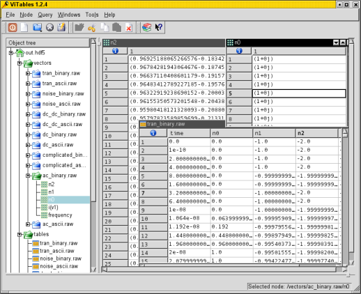
View of an HDF5 file with nddata arrays and metadata inside ViTables.
from pyspecdata import *
init_logging('debug')
a = nddata(r_[0:5:10j], 'x')
a.name('test_data')
try:
    a.hdf5_write('example.h5',getDATADIR(exp_type='Sam'))
except Exception:
    print("file already exists, not creating again -- delete the
    file or node if wanted")
# read the file by the "raw method"
b = nddata_hdf5('example.h5/test_data',
        getDATADIR(exp_type='Sam'))
print("found data:",b)
# or use the find file method
c = find_file('example.h5', exp_type='Sam',
        expno='test_data')
print("found data:",c)
- Parameters:
h5path (str) – Name of the file followed by an optional internal path. The dataset name is taken from the
nameproperty of thenddatainstance.directory (str) – Directory where the HDF5 file lives.
- human_units(scale_data=False)
This function attempts to choose “human-readable” units for axes or y-values of the data. (Terminology stolen from “human readable” file sizes when running shell commands.) This means that it looks at the axis or at the y-values and converts e.g. seconds to milliseconds where appropriate, also multiplying or dividing the data in an appropriate way.
- ift(axes, n=False, tolerance=1e-05, verbose=False, unitary=None, **kwargs)
This performs an inverse Fourier transform along the axes identified by the string or list of strings axes.
- It adjusts normalization and units so that the result conforms to
\(s(t)=\int_{x_{min}}^{x_{max}} \tilde{s}(f) e^{i 2 \pi f t} df\)
pre-IFT, we use the axis to cyclically permute \(f=0\) to the first index
post-IFT, we assume that the data has previously been FT’d If this is the case, passing
shift=Truewill cause an error If this is not the case, passingshift=Truegenerates a standard ifftshiftshift=Nonewill choose True, if and only if this is not the case- Parameters:
pad (int or boolean) –
pad specifies a zero-filling. If it’s a number, then it gives the length of the zero-filled dimension. If it is just True, then the size of the dimension is determined by rounding the dimension size up to the nearest integral power of 2. It uses the start_time ft property to determine the start of the axis. To do this, it assumes that it is a stationary signal (convolved with infinite comb function). The value of start_time can differ from by a non-integral multiple of \(\Delta t\), though the routine will check whether or not it is safe to do this.
- ..note ::
In the code, this is controlled by p2_post (the integral \(\Delta t\) and p2_post_discrepancy – the non-integral.
unitary (boolean (None)) – return a result that is vector-unitary
- property imag
Return the imag component of the data
- indices(axis_name, values)
Return a string of indeces that most closely match the axis labels corresponding to values. Filter them to make sure they are unique.
- inhomog_coords(direct_dim, indirect_dim, tolerance=1e-05, method='linear', plot_name=None, fl=None, debug_kwargs={})
Apply the “inhomogeneity transform,” which rotates the data by \(45^{\circ}\), and then mirrors the portion with \(t_2<0\) in order to transform from a \((t_1,t_2)\) coordinate system to a \((t_{inh},t_{homog})\) coordinate system.
- Parameters:
direct_dim (str) – Label of the direct dimension (typically \(t_2\))
indirect_dim (str) – Label of the indirect dimension (typically \(t_1\))
method ('linear', 'fourier') – The interpolation method used to rotate the data and to mirror the data. Note currently, both use a fourier-based mirroring method.
plot_name (str) – the base name for the plots that are generated
fl (figlist_var) –
debug_kwargs (dict) –
with keys:
- correct_overlap:
if False, doesn’t correct for the overlap error that occurs during mirroring
- integrate(thisaxis, backwards=False, cumulative=False)
Performs an integration – which is similar to a sum, except that it takes the axis into account, i.e., it performs: \(\int f(x) dx\) rather than \(\sum_i f(x_i)\)
Gaussian quadrature, etc, is planned for a future version.
- Parameters:
thisaxis – The dimension that you want to integrate along
cumulative (boolean (default False)) – Perform a cumulative integral (analogous to a cumulative sum) – e.g. for ESR.
backwards (boolean (default False)) – for cumulative integration – perform the integration backwards
- interp(axis, axisvalues, past_bounds=None, return_func=False, **kwargs)
interpolate data values given axis values
- Parameters:
return_func (boolean) – defaults to False. If True, it returns a function that accepts axis values and returns a data value.
- invinterp(axis, values, **kwargs)
interpolate axis values given data values
- item()
like numpy item – returns a number when zero-dimensional
- labels(*args)
label the dimensions, given in listofstrings with the axis labels given in listofaxes – listofaxes must be a numpy np.array; you can pass either a dictionary or a axis name (string)/axis label (numpy np.array) pair
- like(value)
provide “zeros_like” and “ones_like” functionality
- Parameters:
value (float) – 1 is “ones_like” 0 is “zeros_like”, etc.
- linear_shear(along_axis, propto_axis, shear_amnt, zero_fill=True)
the linear shear – see self.shear for documentation
- matchdims(other)
add any dimensions to self that are not present in other
- matrices_3d(also1d=False, invert=False, max_dimsize=1024, downsample_self=False)
returns X,Y,Z,x_axis,y_axis matrices X,Y,Z, are suitable for a variety of mesh plotting, etc, routines x_axis and y_axis are the x and y axes
- mayavi_surf()
use the mayavi surf function, assuming that we’ve already loaded mlab during initialization
- mean(*args, **kwargs)
Take the mean and (optionally) set the error to the standard deviation
- Parameters:
std (bool) – whether or not to return the standard deviation as an error
stderr (bool) – whether or not to return the standard error as an error
- mean_all_but(listofdims)
take the mean over all dimensions not in the list
- mean_weighted(axisname)
perform the weighted mean along axisname (use \(\sigma\) from \(\sigma = `self.get_error() do generate :math:`1/\sigma\) weights) for now, it clears the error of self, though it would be easy to calculate the new error, since everything is linear
unlike other functions, this creates working objects that are themselves nddata objects this strategy is easier than coding out the raw numpy math, but probably less efficient
- meshplot(stride=None, alpha=1.0, onlycolor=False, light=None, rotation=None, cmap=<matplotlib.colors.LinearSegmentedColormap object>, ax=None, invert=False, **kwargs)
takes both rotation and light as elevation, azimuth only use the light kwarg to generate a black and white shading display
- mkd(*arg, **kwargs)
make dictionary format
- name(*arg)
args: .name(newname) –> Name the object (for storage, etc) .name() –> Return the name
- pcolor(fig=None, cmap='viridis', shading='nearest', ax1=None, ax2=None, ax=None, scale_independently=False, vmin=None, vmax=None, human_units=True, force_balanced_cmap=False, handle_axis_sharing=True, mappable_list=None)
generate a pcolormesh and label it with the axis coordinate available from the nddata
- Parameters:
fig (matplotlib figure object) –
cmap (str (default 'viridis')) – cmap to pass to matplotlib pcolormesh
shading (str (default 'nearest')) – the type of shading to pass to matplotlib pcolormesh
ax1 (matplotlib axes object) – where do you want the left plot to go?
ax2 (matplotlib axes object) – where do you want the right plot to go?
ax (matplotlib axes object) – if passed, this is just used for ax1
scale_independently (boolean (default False)) – Do you want each plot to be scaled independently? (If false, the colorbar will have the same limits for all plots)
handle_axis_sharing (boolean (default True)) – Typically, you want the axes to scale together when you zoom – e.g. especially when you are plotting a real and imaginary together. So, this defaults to true to do that. But sometimes, you want to get fancy and, e.g. bind the sharing of many plots together because matplotlib doesn’t let you call sharex/sharey more than once, you need then to tell it not to handle the axis sharing, and to it yourself outside this routine.
mappable_list (list, default []) –
used to scale multiple plots along the same color axis. Used to make all 3x2 plots under a uniform color scale.
List of QuadMesh objects returned by this function.
- Returns:
mappable_list – list of field values for scaling color axis, used to make all 3x2 plots under a uniform color scale
- Return type:
list
- phdiff(axis, return_error=True)
calculate the phase gradient (units: cyc/Δx) along axis, setting the error appropriately
For example, if axis corresponds to a time axis, the result will have units of frequency (cyc/s=Hz).
- plot_labels(labels, fmt=None, **kwargs_passed)
this only works for one axis now
- polyfit(axis, order=1, force_y_intercept=None)
polynomial fitting routine – return the coefficients and the fit .. note:
previously, this returned the fit data as a second argument called formult– you very infrequently want it to be in the same size as the data, though; to duplicate the old behavior, just add the line
formult = mydata.eval_poly(c,'axisname').See also
- Parameters:
axis (str) – name of the axis that you want to fit along (not sure if this is currently tested for multi-dimensional data, but the idea should be that multiple fits would be returned.)
order (int) – the order of the polynomial to be fit
force_y_intercept (double or None) – force the y intercept to a particular value (e.g. 0)
- Returns:
c – a standard numpy np.array containing the coefficients (in ascending polynomial order)
- Return type:
np.ndarray
- random_mask(axisname, threshold=np.float64(0.36787944117144233), inversion=False)
generate a random mask with about ‘threshold’ of the points thrown out
- property real
Return the real component of the data
- register_axis(arg, nearest=None)
Interpolate the data so that the given axes are in register with a set of specified values. Does not change the spacing of the axis labels.
It finds the axis label position that is closest to the values given in arg, then interpolates (Fourier/sinc method) the data onto a new, slightly shifted, axis that passes exactly through the value given. To do this, it uses
.ft_new_startpoint()and uses.set_ft_prop()to override the “not aliased” flag.- Parameters:
arg (dict (key,value = str,double)) – A list of the dimensions that you want to place in register, and the values you want them registered to.
nearest (bool, optional) – Passed through to ft_new_startpoint
- reorder(*axes, **kwargs)
Reorder the dimensions the first arguments are a list of dimensions
- Parameters:
*axes (str) – Accept any number of arguments that gives the dimensions, in the order that you want thee.
first (bool) – (default True) Put this list of dimensions first, while False puts them last (where they then come in the order given).
- run(*args)
run a standard numpy function on the nddata:
d.run(func,'axisname')will run function func (e.g. a lambda function) along axis named ‘axisname’d.run(func)will run function func on the datain general: if the result of func reduces a dimension size to 1, the ‘axisname’ dimension will be “popped” (it will not exist in the result) – if this is not what you want, use
run_nopop
- run_avg(thisaxisname, decimation=20, centered=False)
a simple running average
- secsy_transform(direct_dim, indirect_dim, has_indirect=True, method='fourier', truncate=True)
Shift the time-domain data backwards by the echo time.
As opposed to
secsy_transform_manual, this calls on onskew, rather than directly manipulating the phase of the function, which can lead to aliasing.- Parameters:
has_indirect (bool) –
(This option is largely specific to data loaded by
acert_hdf5)Does the data actually have an indirect dimension? If not, assume that there is a constant echo time, that can be retrieved with
.get_prop('te').truncate (bool) – If this is set, register_axis <pyspecdata.axis_manipulation.register_axis> to \(t_{direct}=0\), and then throw out the data for which \(t_{direct}<0\).
method (str) – The shear method (linear or fourier).
- secsy_transform_manual(direct_dim, indirect_dim, has_indirect=True, truncate=False)
Shift the time-domain data backwards by the echo time. As opposed to
secsy_transform, this directlly manipulates the phase of the function, rather than calling onskew.- Parameters:
has_indirect (bool) –
(This option is largely specific to data loaded by
acert_hdf5)Does the data actually have an indirect dimension? If not, assume that there is a constant echo time, that can be retrieved with
.get_prop('te').truncate (bool) – If this is set, register_axis <pyspecdata.axis_manipulation.register_axis> to \(t_{direct}=0\), and then throw out the data for which \(t_{direct}<0\).
- set_error(*args)
set the errors: either
set_error(‘axisname’,error_for_axis) or set_error(error_for_data)
error_for_data can be a scalar, in which case, all the data errors are set to error_for_data
Todo
several options below – enumerate them in the documentation
- set_ft_initial(axis, which_domain='t', shift=True)
set the current domain as the ‘initial’ domain, the following three respects:
Assume that the data is not aliased, since aliasing typically only happens as the result of an FT
Label the FT property initial_domain as “time-like” or “frequency-like”, which is used in rendering the axes when plotting.
Say whether or not we will want the FT to be shifted so that it’s center is at zero, or not.
More generally, this is achieved by setting the FT “start points” used to determine the windows on the periodic functions.
- Parameters:
shift (True) – When you (i)ft away from this domain, shift
- set_ft_prop(axis, propname=None, value=True)
Sets the FT property given by propname. For both setting and getting, None is equivalent to an unset value if propname is a boolean, and value is True (the default), it’s assumed that propname is actually None, and that value is set to the propname argument (this allows us to set the FT property more easily)
- set_plot_color_next()
set the plot color associated with this dataset to the next one in the global color cycle
Note that if you want to set the color cycle to something that’s not the matplotlib default cycle, you can modify pyspecdata.core.default_cycler in your script.
- set_prop(*args, **kwargs)
set a ‘property’ of the nddata This is where you can put all unstructured information (e.g. experimental parameters, etc)
Accepts:
a single string, value pair
a dictionary
a set of keyword arguments
- set_to(otherinst)
Set data inside the current instance to that of the other instance.
Goes through the list of attributes specified in copy, and assigns them to the element of the current instance.
This is to be used:
for constructing classes that inherit nddata with additional methods.
for overwriting the current data with the result of a slicing operation
- set_axis(*args)
set or alter the value of the coordinate axis
Can be used in one of several ways:
self.set_axis('axisname', values): just sets the valuesself.set_axis('axisname', '#'): justnumber the axis in numerically increasing order, with integers, (e.g. if you have smooshed it from a couple other dimensions.)
self.fromaxis('axisname',inputfunc): take the existing function,apply inputfunc, and replace
self.fromaxis(inputsymbolic): Evaluate inputsymbolic and loadthe result into the axes, appropriately
- shear(along_axis, propto_axis, shear_amnt, zero_fill=True, start_in_conj=False, method='linear')
Shear the data \(s\):
\(s(x',y,z) = s(x+ay,y,z)\)
where \(x\) is the altered_axis and \(y\) is the propto_axis. (Actually typically 2D, but \(z\) included just to illustrate other dimensions that aren’t involved)
- Parameters:
method ({'fourier','linear'}) –
- fourier
Use the Fourier shift theorem (i.e., sinc interpolation). A shear is equivalent to the following in the conjugate domain:
..math: tilde{s}(f_x,f’_y,z) = tilde{s}(f_x,f_y-af_x,f_z)
Because of this, the algorithm also automatically extend`s the data in `f_y axis. Equivalently, it increases the resolution (decreases the interval between points) in the propto_axis dimension. This prevents aliasing in the conjugate domain, which will corrupt the data w.r.t. successive transformations. It does this whether or not zero_fill is set (zero_fill only controls filling in the “current” dimension)
- linear
Use simple linear interpolation.
altered_axis (str) – The coordinate for which data is altered, i.e. ..math: x such that ..math: f(x+ay,y).
by_amount (double) – The amount of the shear (..math: a in the previous)
propto_axis (str) – The shift along the altered_axis dimension is proportional to the shift along propto_axis. The position of data relative to the propto_axis is not changed. Note that by the shift theorem, in the frequency domain, an equivalent magnitude, opposite sign, shear is applied with the propto_axis and altered_axis dimensions flipped.
start_in_conj ({False, True}, optional) –
Defaults to False
For efficiency, one can replace a double (I)FT call followed by a shear call with a single shear call where start_in_conj is set.
self before the call is given in the conjugate domain (i.e., \(f\) vs. \(t\)) along both dimensions from the one that’s desired. This means: (1) self after the function call transformed into the conjugate domain from that before the call and (2) by_amount, altered_axis, and propto_axis all refer to the shear in the conjugate domain that the data is in at the end of the function call.
- smoosh(dimstocollapse, dimname=0, noaxis=False)
Collapse (smoosh) multiple dimensions into one dimension.
- Parameters:
dimstocollapse (list of strings) – the dimensions you want to collapse to one result dimension
dimname (None, string, integer (default 0)) –
if dimname is:
None: create a new (direct product) name,
- a number: an index to the
dimstocollapselist. The resulting smooshed dimension will be named
dimstocollapse[dimname]. Because the default is the number 0, the new dimname will be the first dimname given in the list.
- a number: an index to the
- a string: the name of the resulting smooshed dimension (can be
part of the
dimstocollapselist or not)
noaxis (bool) – if set, then just skip calculating the axis for the new dimension, which otherwise is typically a complicated record array
- Returns:
self (nddata) – the dimensions dimstocollapse are smooshed into a single dimension, whose name is determined by dimname. The axis for the resulting, smooshed dimension is a structured np.array consisting of two fields that give the labels along the original axes.
..todo:: – when we transition to axes that are stored using a slice/linspace-like format, allow for smooshing to determine a new axes that is standard (not a structured np.array) and that increases linearly.
- spline_lambda(s_multiplier=None)
For 1D data, returns a lambda function to generate a Cubic Spline.
- Parameters:
s_multiplier (float) – If this is specified, then use a smoothing BSpline, and set “s” in scipy to the len(data)*s_multiplier
- Returns:
nddata_lambda – Takes one argument, which is an array corresponding to the axis coordinates, and returns an nddata.
- Return type:
lambda function
- squeeze(return_dropped=False)
squeeze singleton dimensions
- Parameters:
return_dropped (bool (default False)) – return a list of the dimensions that were dropped as a second argument
- Returns:
self
return_dropped (list) – (optional, only if return_dropped is True)
- sum(axes)
calculate the sum along axes, also transforming error as needed
- svd(todim, fromdim)
Singular value decomposition. Original matrix is unmodified.
Note
Because we are planning to upgrade with axis objects, FT properties, axis errors, etc, are not transferred here. If you are using it when this note is still around, be sure to .copy_props(
Also, error, units, are not currently propagated, but could be relatively easily!
If
>>> U, Sigma, Vh = thisinstance.svd()
then
U,Sigma, andVhare nddata such thatresultin>>> result = U @ Sigma @ Vh
will be the same as
thisinstance. Note that this relies on the fact that nddata matrix multiplication doesn’t care about the ordering of the dimensions (see :method:`~pyspecdata.core.dot`). The vector space that contains the singular values is called ‘SV’ (see more below).- Parameters:
fromdim (str) – This dimension corresponds to the columns of the matrix that is being analyzed by SVD. (The matrix transforms from the vector space labeled by
fromdimand into the vector space labeled bytodim).todim (str) – This dimension corresponds to the rows of the matrix that is being analyzed by SVD.
- Returns:
U (nddata) – Has dimensions (all other dimensions) × ‘todim’ × ‘SV’, where the dimension ‘SV’ is the vector space of the singular values.
Sigma (nddata) – Has dimensions (all other dimensions) × ‘SV’. Only non-zero
Vh (nddata) – Has dimensions (all other dimensions) × ‘SV’ × ‘fromdim’,
- to_ppm(axis='t2', freq_param='SFO1', offset_param='OFFSET')
Function that converts from Hz to ppm using Bruker parameters
- Parameters:
axis (str, 't2' default) – label of the dimension you want to convert from frequency to ppm
freq_param (str) – name of the acquisition parameter that stores the carrier frequency for this dimension
offset_param (str) – name of the processing parameter that stores the offset of the ppm reference (TMS, DSS, etc.)
todo:: (..) –
Figure out what the units of PHC1 in Topspin are (degrees per what??), and apply those as well.
make this part of an inherited bruker class
- unitify_axis(axis_name, is_axis=True)
this just generates an axis label with appropriate units
- unset_prop(arg)
remove a ‘property’