Calculation of the Covariance Matrix

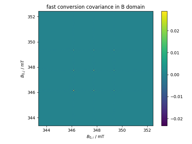
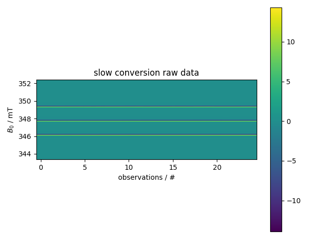
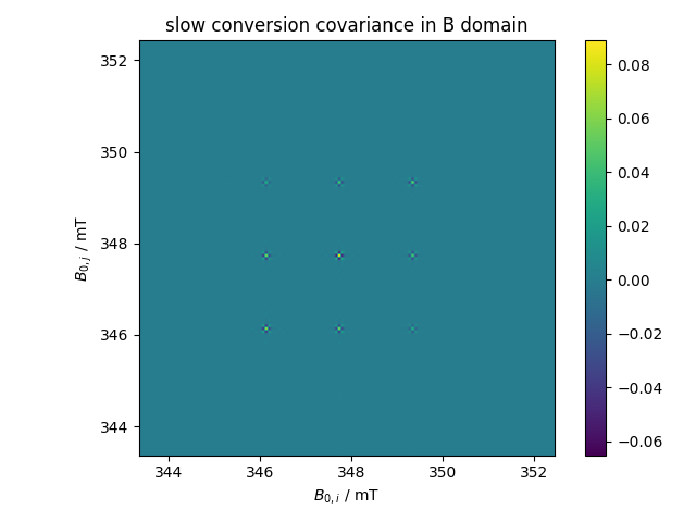
After rescaling plots, the covariance matrix is calculated and then plotted for a 2D Field experiment (spectra as a function of field with multiple collections or “Times”)

• 
• 
• 
• 
• 
• 

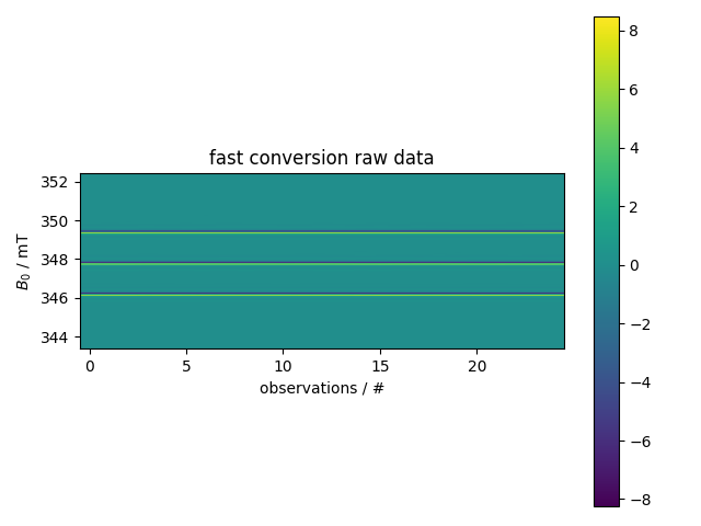
1: fast conversion raw data |||('s', 'mT')
2: fast conversion covariance in B domain |||('mT', 'mT')
3: fast conversion Covariance in U domain |||('kcyc · (T)$^{-1}$', 'kcyc · (T)$^{-1}$')
4: slow conversion raw data |||('s', 'mT')
5: slow conversion covariance in B domain |||('mT', 'mT')
6: slow conversion Covariance in U domain |||('kcyc · (T)$^{-1}$', 'kcyc · (T)$^{-1}$')

from pyspecdata import *
from pylab import *

fieldaxis = "$B_0$"
exp_type = "francklab_esr/romana"
with figlist_var() as fl:
    for filenum, (thisfile, fl.basename) in enumerate([
        (
            re.escape("250123_TEMPOL_100uM_AG_Covariance_2D.DSC"),
            "fast conversion",
        ),
        (
            re.escape("250123_TEMPOL_100uM_AG_Covariance_2D_cc12.DSC"),
            "slow conversion",
        ),
    ]):
        d = find_file(thisfile, exp_type=exp_type)["harmonic", 0]
        d.set_units(fieldaxis, "T").setaxis(fieldaxis, lambda x: x * 1e-4)
        d.rename("Time", "observations")
        d.reorder([fieldaxis,"observations"])
        fl.next("raw data")
        fl.image(d)
        fl.next("covariance in B domain")
        # we do this first, because if we were to ift to go to u domain and
        # then ft back, we would introduce a complex component to our data
        fl.image(d.C.cov_mat("observations"))
        d.ift(fieldaxis, shift=True)
        fl.next("Covariance in U domain")
        fl.image(
            d.cov_mat("observations").run(abs)
        )  # this time, do not spin up an extra copy of the data