Error and units example

Here is a simple example of errors and unit propagation

Notice that the base nddata class supplies error and propagation similar to uncertainty-type libraries.

For the units, pint is doing the heavy lifting here.

import pyspecdata as psd
from numpy import r_
import matplotlib.pyplot as plt

As a simple example, say that we perform several measurements of a volume (not sure physically why we would have such variability, but let’s roll with it to keep the example simple!)

vol = psd.nddata(r_[1.10, 1.11, 1.02, 1.03, 1.00, 1.05]).set_units("L")

Similarly, let’s take some measurements of the weight of a solute!

weight = psd.nddata(r_[2.10, 2.61, 2.002, 2.73, 2.33, 2.69]).set_units("μg")

To test our error propagation below, we’re going to divide the two arrays here – because the variability of this number should be somewhat similar to the propagated error below (though of course, there is a statistical difference, and doing the two things does mean something different). Notice how, during string conversion, we always give the standard error 2 significant figures, and then base the significant figures of the number on the error.

conc_indiv = weight / vol
conc_indiv.mean(stderr=True)
print(conc_indiv)

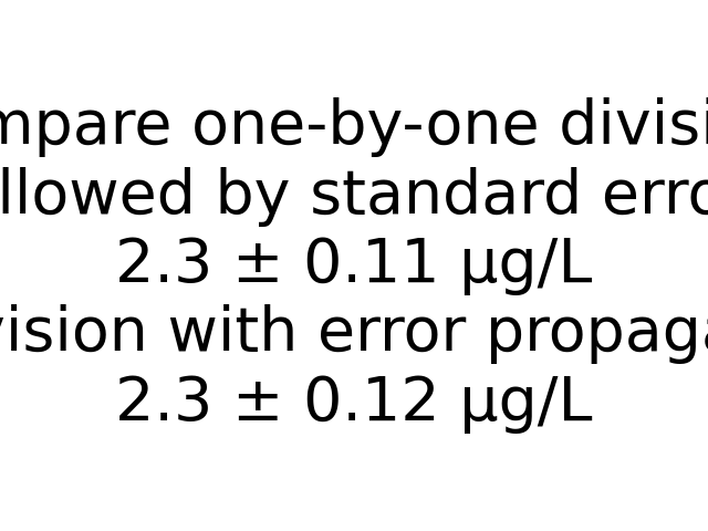
2.3 ± 0.11 µg/L

We take the mean, allowing it to accumulate the standard error. (See comment above about significant figures.)

vol.mean(stderr=True)
print(vol)

weight.mean(stderr=True)
print(weight)

print(weight / vol)

# Because we want this to show up in sphinx gallery, we have
# to make some type of figure

fig = plt.figure()
text = plt.Text(
    x=0.5,
    y=0.5,
    text=(
        "Compare one-by-one division,\nfollowed by standard"
        f" error:\n{conc_indiv}\nto division with error"
        f" propagation:\n{weight/vol}"
    ),
    fontsize=40,
    ha="center",
    va="center",
)
fig.add_artist(text)
fig.tight_layout()
plt.show()

1.05 ± 0.017 L
2.4 ± 0.12 µg
2.3 ± 0.12 µg/L