Simple Convolution Example

Since we use convolution a bit for signal analysis, test it here.

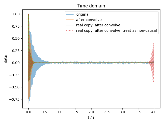
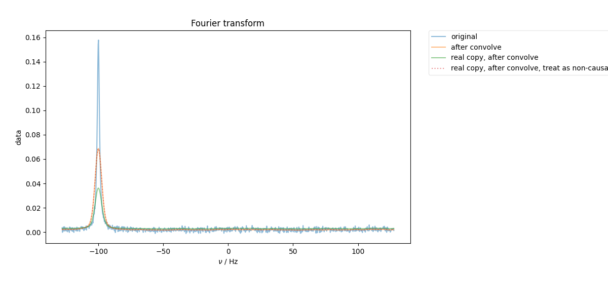
This also demonstrates the point that, when performing convolution, it’s important to distinguish between signals that are “causal” (like an FID – consisting of real and imag that are Hermite transform pairs) vs. “non-causal” (e.g. take the real part or the energy of a causal signal, or analyze a noise PSD). We show the time-domain signal by way of explanation as to how these are treated differently.

• 
• 

1: Time domain |||s
2: Fourier transform |||Hz

from pylab import *
from pyspecdata import *
t = nddata(r_[0:4:1024j],'t').set_units('t','s')
signal = exp(-1j*2*pi*100*t-20*t/pi)
signal.add_noise(0.01)
with figlist_var() as fl:
    fl.next('Time domain')
    fl.plot(signal, label='original')
    fl.next('Fourier transform', legend=True)
    signal.ft('t', shift=True)
    signal_real_copy = signal.real
    signal_real_copy_noncausal = signal.real
    fl.plot(signal, label='original')
    signal.convolve('t',5)
    signal_real_copy.convolve('t',5)
    signal_real_copy_noncausal.convolve('t',5, enforce_causality=False)
    fl.plot(signal, label='after convolve')
    fl.plot(signal_real_copy, label='real copy, after convolve')
    fl.plot(signal_real_copy_noncausal, ':', label='real copy, after convolve, treat as non-causal')
    fl.next('Time domain')
    signal.ift('t')
    signal_real_copy.ift('t')
    signal_real_copy_noncausal.ift('t')
    fl.plot(signal, label='after convolve')
    fl.plot(signal_real_copy, label='real copy, after convolve')
    fl.plot(signal_real_copy_noncausal, ':', label='real copy, after convolve, treat as non-causal')