BSA UV-Vis Calibration

This example is specifically designed to process data from a BSA calibration curve lab exercise.

To run the curve for your data:

• Make sure the data is stored on google drive in the exp_data/UV_Vis/BSA_calib directory, and your computer is set up so that your _pyspecdata file points to google drive.

• Just make a copy of this file, change the name of the BSW file to point to your data

• Then edit the table inside the OrderedDict below so that it gives the correct labels and scan names for all the spectra in your run.

• edit the background parameter below so that it points to the scan that you want to function as your baseline/background. - We would rather record the raw absorbance values, rather than rely on

  the spectrometer to subtract and hide the absorbance values of our baseline.

• 
• 

the experiments present in this file are: dict_keys(['UP_H2O', 'K-PBSbuffer', 'J-0p0078%BSA', 'H-0p0156%BSA', 'G-0p0234%BSA1', 'F-0p0311%BSA', 'G-0p0234%BSA_actual', 'E-0p0389%BSA', 'D-0p0466%BSA', 'C-0p0544%BSA', 'B-0p0622%BSA', 'A-0p0700%BSA'])
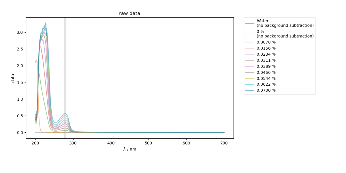
1: raw data |||nm
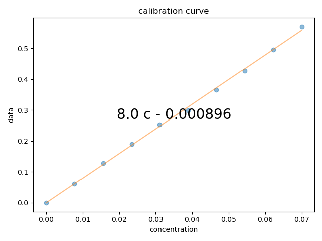
2: calibration curve |||None

from pylab import *
from pyspecdata import *
import numpy as np
import matplotlib.pyplot as plt
from collections import OrderedDict
import sympy as sp

# {{{ some constants
wv = "$\\lambda$"
wv_range = (276, 281)  # range of wavelengths we consider to be our peak
# }}}

# HERE we get dictionaries of nddata
dataWKBSA = find_file(
    "221110_BSAexerciseWK_0p07-0percentBSAcalibration.BSW", exp_type="UV_Vis/BSA_Exercise"
)
print("the experiments present in this file are:", dataWKBSA.keys())
# from our notebook, we get the following info
# think of this like a dictionary -- what is the sample called (on the left)
# and what's its scan label (on the right).  **Ideally** the scan labels
# shouldn't be this complicated -- they should just be single letters, as noted
# in the protocol.
#
# Code below expects that when the label/key below is a concentration, it has a % symbol
list_of_runs = OrderedDict(
    [
        ("Water", "UP_H2O"),
        ("0 %", "K-PBSbuffer"),
        ("0.0078 %", "J-0p0078%BSA"),
        ("0.0156 %", "H-0p0156%BSA"),
        ("0.0234 %", "G-0p0234%BSA_actual"),
        ("0.0311 %", "F-0p0311%BSA"),
        ("0.0389 %", "E-0p0389%BSA"),
        ("0.0466 %", "D-0p0466%BSA"),
        ("0.0544 %", "C-0p0544%BSA"),
        ("0.0622 %", "B-0p0622%BSA"),
        ("0.0700 %", "A-0p0700%BSA"),
    ]
)
background = (
    "0 %"  # this is the label of the thing we want to subtract as the background
)
with figlist_var() as fl:
    # {{{ first, just show the raw data and the region of the spectrum that we intend to slice
    bg_data = dataWKBSA[list_of_runs[background]]
    fl.next("raw data", legend=True)
    plt.axvspan(wv_range[0], wv_range[1], color="k", alpha=0.1)
    for thislabel, thisscan in list_of_runs.items():
        if thislabel in [background, "Water"]:
            fl.plot(
                dataWKBSA[thisscan],
                label=thislabel + "\n(no background subtraction)",
                alpha=0.5,
            )
        else:
            fl.plot(dataWKBSA[thisscan] - bg_data, label=thislabel, alpha=0.5)
    # }}}
    # {{{ pull a list of all of the spectra whose labels express a concentration
    #     (percentage), as well as an array of floating point values for the
    #     corresponding concentrations
    conc_labels = [k for k, v in list_of_runs.items() if "%" in k]
    conc_values = array([float(j.replace("%", "")) for j in conc_labels])
    bg_data = dataWKBSA[list_of_runs[background]]
    all_data = concat(
        [dataWKBSA[list_of_runs[k]] - bg_data for k in conc_labels], "concentration"
    ).setaxis("concentration", conc_values)
    # }}}
    # {{{ now, gather the data in to a 2D array, so that I can just average the peak and plot the calibration curve
    A280 = all_data[wv:wv_range].mean(wv)
    fl.next("calibration curve")
    fl.plot(A280, "o")
    c = A280.polyfit("concentration", order=1)
    fl.plot(A280.eval_poly(c, "concentration"))
    # }}}
    # {{{ use sympy to print the fit equation
    conc_symb = sp.symbols("c", real=True)
    expr = sum([conc_symb ** j * sp.Float(c[j], 3) for j in range(len(c))])
    plt.text(
        0.5,
        0.5,
        sp.latex(expr),
        transform=gca().transAxes,
        va="center",
        ha="center",
        size=20,
    )
    # }}}