2D ILT

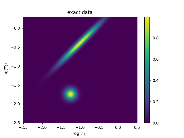
Here, we’re going to provide a few demonstrations of the ILT functionality. Let’s start with Fig 1.10 in A. Beaton’s thesis, which is based off the figures in Venkataramanan.

from pylab import (
    figure,
    title,
    show,
    linspace,
    logspace,
    log10,
    exp,
    sqrt,
    rcParams,
)
import numpy as np
from pyspecdata import nddata, image

rcParams["image.aspect"] = "auto"  # needed for sphinx gallery
# sphinx_gallery_thumbnail_number = 2

NT1 = 300  # Number of T1 values
NT2 = 300  # Number of T2 values
LT1_name = r"$\log(T_1)$"
LT1 = nddata(linspace(-2.5, 0.5, NT1), LT1_name)
LT2_name = r"$\log(T_2)$"
LT2 = nddata(linspace(-2.5, 0.3, NT2), LT2_name)
mu = [-1.25, -1.75]
sigma = [0.1, 0.1]
exact_data = exp(
    -((LT1 - mu[0]) ** 2) / 2 / sigma[0] ** 2
    - (LT2 - mu[1]) ** 2 / 2 / sigma[1] ** 2
)
slanted_coord1 = (LT1 + LT2) / sqrt(2)
slanted_coord2 = (LT2 - LT1) / sqrt(2)
mu = [-1.0, -0.4]
mu = [  # convert to slanted coords
    (mu[0] + mu[1]) / sqrt(2),
    (mu[1] - mu[0]) / sqrt(2),
]
sigma = [0.5, 0.05]  # in slanted
exact_data += exp(
    -((slanted_coord1 - mu[0]) ** 2) / 2 / sigma[0] ** 2
    - (slanted_coord2 - mu[1]) ** 2 / 2 / sigma[1] ** 2
)
exact_data.reorder(LT2_name)  # T₂ along y axis

figure(1)
title("exact data")
image(exact_data)

<matplotlib.image.AxesImage object at 0x7f2714062b90>

Now add the experimental decay dimensions (\(\tau_1\) and \(\tau_2\))

tau1 = nddata(logspace(log10(5.0e-4), log10(4), 30), "tau1")
tau2 = nddata(linspace(5.0e-4, 3.8, 1000), "tau2")

Pre-allocate the \(\tau_1\times\tau_2\) result via ndshape’s alloc, inline

simulated_data = (tau1.shape | tau2.shape).alloc(dtype=np.float64)
simulated_data.reorder("tau2")  # T₂ along y axis

array([[0., 0., 0., ..., 0., 0., 0.],
       [0., 0., 0., ..., 0., 0., 0.],
       [0., 0., 0., ..., 0., 0., 0.],
       ...,
       [0., 0., 0., ..., 0., 0., 0.],
       [0., 0., 0., ..., 0., 0., 0.],
       [0., 0., 0., ..., 0., 0., 0.]])
    dimlabels=['tau2', 'tau1']
    axes={`tau2':None
                    +/-None,
            `tau1':None
                    +/-None}

pySpecData makes it easy to construct fake data like this. Typically this is very easy, but here, we must contend with the fact that we are memory-limited, so if we want a highly resolved fit basis, we need to chunk up the calculation. Nonetheless, pySpecData still makes that easy: let’s see how!

Block sizes (tune to available RAM)

bLT1 = 20
bLT2 = 20

Loop over LT1 and LT2 in blocks, vectorized over \(\tau_{1}\) and \(\tau_{2}\) dims each time

\[ \begin{align}\begin{aligned}T_1 = 10^{\log(T_1)}\\R_1 = 10^{-\log(T_1)}\\\ln(R_1) = -\log(T_1) \ln(10)\end{aligned}\end{align} \]

print(
    "Generating the fake data can take some time.  I need to loop a"
    f" calculation in chunks over a {LT1.shape[LT1_name]} ×"
    f" {LT2.shape[LT2_name]} grid"
)
for i in range(0, LT1.shape[LT1_name], bLT1):
    LT1_blk = LT1[LT1_name, slice(i, i + bLT1)]
    B1 = 1 - 2 * exp(-tau1 / 10**LT1_blk)  # dims: (tau1, LT1_blk)
    for j in range(0, LT2.shape[LT2_name], bLT2):
        print(i, j)
        LT2_blk = LT2[LT2_name, slice(j, j + bLT2)]
        B2 = exp(-tau2 / 10**LT2_blk)  # dims: (tau2, LT2_blk)
        # Extract matching block of exact_data
        data_blk = exact_data[LT1_name, slice(i, i + bLT1)][
            LT2_name, slice(j, j + bLT2)
        ]  # dims: (tau1, tau2, LT1_blk, LT2_blk)
        # Multiply, sum out both LT axes, and accumulate
        simulated_data += (B2 * B1 * data_blk).real.sum(LT1_name).sum(LT2_name)
print("done generating")

Generating the fake data can take some time.  I need to loop a calculation in chunks over a 300 × 300 grid
0 0
0 20
0 40
0 60
0 80
0 100
0 120
0 140
0 160
0 180
0 200
0 220
0 240
0 260
0 280
20 0
20 20
20 40
20 60
20 80
20 100
20 120
20 140
20 160
20 180
20 200
20 220
20 240
20 260
20 280
40 0
40 20
40 40
40 60
40 80
40 100
40 120
40 140
40 160
40 180
40 200
40 220
40 240
40 260
40 280
60 0
60 20
60 40
60 60
60 80
60 100
60 120
60 140
60 160
60 180
60 200
60 220
60 240
60 260
60 280
80 0
80 20
80 40
80 60
80 80
80 100
80 120
80 140
80 160
80 180
80 200
80 220
80 240
80 260
80 280
100 0
100 20
100 40
100 60
100 80
100 100
100 120
100 140
100 160
100 180
100 200
100 220
100 240
100 260
100 280
120 0
120 20
120 40
120 60
120 80
120 100
120 120
120 140
120 160
120 180
120 200
120 220
120 240
120 260
120 280
140 0
140 20
140 40
140 60
140 80
140 100
140 120
140 140
140 160
140 180
140 200
140 220
140 240
140 260
140 280
160 0
160 20
160 40
160 60
160 80
160 100
160 120
160 140
160 160
160 180
160 200
160 220
160 240
160 260
160 280
180 0
180 20
180 40
180 60
180 80
180 100
180 120
180 140
180 160
180 180
180 200
180 220
180 240
180 260
180 280
200 0
200 20
200 40
200 60
200 80
200 100
200 120
200 140
200 160
200 180
200 200
200 220
200 240
200 260
200 280
220 0
220 20
220 40
220 60
220 80
220 100
220 120
220 140
220 160
220 180
220 200
220 220
220 240
220 260
220 280
240 0
240 20
240 40
240 60
240 80
240 100
240 120
240 140
240 160
240 180
240 200
240 220
240 240
240 260
240 280
260 0
260 20
260 40
260 60
260 80
260 100
260 120
260 140
260 160
260 180
260 200
260 220
260 240
260 260
260 280
280 0
280 20
280 40
280 60
280 80
280 100
280 120
280 140
280 160
280 180
280 200
280 220
280 240
280 260
280 280
done generating

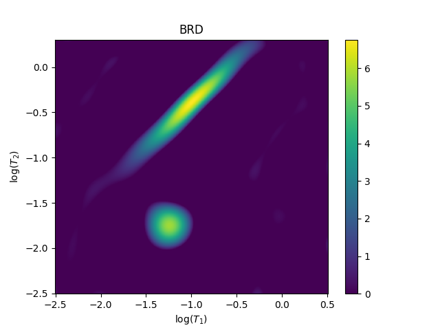
simulated_data now holds the \(\tau_1\times\tau_2\) synthetic data. So, add noise, and scale data so that noise has norm of 1

simulated_data.add_noise(0.1)
simulated_data /= 0.1

Use BRD to find the value of $lambda$ ($alpha$). Note that BRD assumes that you have scaled your data so that the stdev of the noise is 1.0.

simulated_data.nnls(
    ("tau1", "tau2"),
    (LT1, LT2),
    (
        lambda tau1, LT1: 1 - 2 * exp(-tau1 * 10**-LT1),
        lambda tau2, LT2: exp(-tau2 * 10**-LT2),
    ),
    l="BRD",
)

figure(2)
title("BRD")
image(simulated_data)

show()