1D BRD regularization

For 1D BRD, adapted mainly from Venkataramanan 2002 but checked against a compiled stacked regularization that uses Lawson-Hansen.

Note that one of the unit tests essentially tests that this example behaves as expected.

• 
• 

----------  logging output to /home/jmfranck/pyspecdata.0.log  ----------
[(25, 'vd'), (100, '$\\log(T_1)$')]
[(100, '$\\log(T_1)$')]
[(25, 'vd')]
*** *** ***
[(25, 'vd')]
[(100, '$\\log(T_1)$')]
*** *** ***
--> nnls.py(172):pyspecdata.matrix_math                 nnls 2025-07-08 15:37:33,408
INFO: argcheck done
--> nnls.py(291):pyspecdata.matrix_math                 nnls 2025-07-08 15:37:33,416
INFO: S1 is [4.32594139e+01 1.14067699e+01 5.27410398e+00 2.31565579e+00
 6.82140197e-01 2.07917079e-01 5.68093757e-02 1.53070136e-02
 3.75635882e-03 8.94520237e-04 1.95762142e-04 4.11592621e-05
 7.98652315e-06 1.47596130e-06 2.51772342e-07 4.05185112e-08
 5.99364462e-09 8.26213697e-10 1.03618610e-10 1.18847096e-11
 1.21391608e-12 1.09570779e-13 8.58076129e-15 1.58097699e-15
 7.13572588e-16] so I'm going to 6 based on default_cut of 0.001
--> nnls.py(370):pyspecdata.matrix_math                 nnls 2025-07-08 15:37:33,417
INFO: about to run venk(6, 100) (6,)
--> nnls.py(172):pyspecdata.matrix_math                 nnls 2025-07-08 15:37:33,418
INFO: argcheck done
--> nnls.py(291):pyspecdata.matrix_math                 nnls 2025-07-08 15:37:33,425
INFO: S1 is [4.32594139e+01 1.14067699e+01 5.27410398e+00 2.31565579e+00
 6.82140197e-01 2.07917079e-01 5.68093757e-02 1.53070136e-02
 3.75635882e-03 8.94520237e-04 1.95762142e-04 4.11592621e-05
 7.98652315e-06 1.47596130e-06 2.51772342e-07 4.05185112e-08
 5.99364462e-09 8.26213697e-10 1.03618610e-10 1.18847096e-11
 1.21391608e-12 1.09570779e-13 8.58076129e-15 1.58097699e-15
 7.13572588e-16] so I'm going to 6 based on default_cut of 0.001
--> nnls.py(172):pyspecdata.matrix_math                 nnls 2025-07-08 15:37:33,428
INFO: argcheck done
--> nnls.py(291):pyspecdata.matrix_math                 nnls 2025-07-08 15:37:33,435
INFO: S1 is [4.32594139e+01 1.14067699e+01 5.27410398e+00 2.31565579e+00
 6.82140197e-01 2.07917079e-01 5.68093757e-02 1.53070136e-02
 3.75635882e-03 8.94520237e-04 1.95762142e-04 4.11592621e-05
 7.98652315e-06 1.47596130e-06 2.51772342e-07 4.05185112e-08
 5.99364462e-09 8.26213697e-10 1.03618610e-10 1.18847096e-11
 1.21391608e-12 1.09570779e-13 8.58076129e-15 1.58097699e-15
 7.13572588e-16] so I'm going to 6 based on default_cut of 0.001
[(25, 'vd'), (100, '$\\log(T_1)$')]
true mean: 0.16499997337102065 ± 0.3576690429197919
opt. λ mean: 0.9013864830113146 ± 1.709683940073894
BRD mean: 0.9318763536449894 ± 1.5859823021148707

from matplotlib.pyplot import figure, show, title, legend, axvline, rcParams
from numpy import linspace, exp, zeros, eye, logspace, r_, sqrt, pi, std
from pylab import linalg
from pyspecdata import nddata, init_logging, plot
from scipy.optimize import nnls
from numpy.random import seed

rcParams["image.aspect"] = "auto"  # needed for sphinx gallery
# sphinx_gallery_thumbnail_number = 2

seed(1234)
init_logging("debug")
vd_list = nddata(linspace(5e-4, 10, 25), "vd")
t1_name = r"$\log(T_1)$"
logT1 = nddata(r_[-4:2:100j], t1_name)


mu1 = 0.5
sigma1 = 0.3
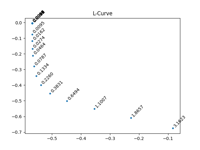
L_curve_l = 0.036  # read manually off of plot
plot_Lcurve = True
true_F = (
    1 / sqrt(2 * pi * sigma1**2) * exp(-((logT1 - mu1) ** 2) / 2 / sigma1**2)
)


K = 1.0 - 2 * exp(-vd_list / 10 ** (logT1))

K.reorder("vd")  # make sure vd along rows
print(K.shape)
print(true_F.shape)

M = K @ true_F  # the fake data
print(M.shape)
# M.setaxis('vd',y_axis)
M.add_noise(0.2)
M /= 0.2  # this is key -- make sure that the noise variance is 1, for BRD

# this is here to test the integrated 1D-BRD (for pyspecdata)
print("*** *** ***")
print(M.shape)
print(logT1.shape)
print("*** *** ***")
solution = M.C.nnls(
    "vd", logT1, lambda x, y: 1 - 2 * exp(-x / 10 ** (y)), l="BRD"
)
solution_confirm = M.C.nnls(
    "vd",
    logT1,
    lambda x, y: 1 - 2 * exp(-x / 10 ** (y)),
    l=sqrt(solution.get_prop("opt_alpha")),
)


def nnls_reg(K, b, val):
    b_prime = r_[b, zeros(K.shape[1])]
    x, _ = nnls(A_prime(K, val), b_prime)
    return x


# generate the A matrix, which should have form of the original kernel and then
# an additional length corresponding to size of the data dimension, where
# smothing param val is placed
def A_prime(K, val):
    dimension = K.shape[1]
    A_prime = r_[K, val * eye(dimension)]
    return A_prime


if plot_Lcurve:
    # {{{ L-curve
    # solution matrix for l different lambda values
    x = M.real.C.nnls(
        "vd",
        logT1,
        lambda x, y: (1.0 - 2 * exp(-x / 10 ** (y))),
        l=sqrt(
            logspace(-10, 1, 25)
        ),  # adjusting the left number will adjust the right side of L-curve
    )
    # norm of the residual (data - soln)
    # norm of the solution (taken along the fit axis)
    x.run(linalg.norm, t1_name)

    # From L-curve
    figure()
    axvline(x=L_curve_l, ls="--")
    plot(x)
    # }}}

# generate data vector for smoothing

print(K.shape)
L_opt_vec = nnls_reg(K.data, M.data.squeeze(), L_curve_l)

figure()
title("ILT distributions")
L_opt_vec = nddata(L_opt_vec, t1_name).copy_axes(true_F)
normalization = solution.data.max() / true_F.data.max()
plot(true_F * normalization, label="True")
print(
    "true mean:",
    true_F.C.mean(t1_name).item(),
    "±",
    true_F.run(std, t1_name).item(),
)
plot(L_opt_vec, label="L-Curve")
print(
    "opt. λ mean:",
    L_opt_vec.C.mean(t1_name).item(),
    "±",
    L_opt_vec.run(std, t1_name).item(),
)
plot(solution, ":", label="pyspecdata-BRD")
plot(
    solution_confirm,
    "--",
    label=rf"manual BRD $\alpha={solution.get_prop('opt_alpha'):#0.2g}$",
    alpha=0.5,
)
print(
    "BRD mean:",
    solution.C.mean(t1_name).item(),
    "±",
    solution.run(std, t1_name).item(),
)
legend()
show()