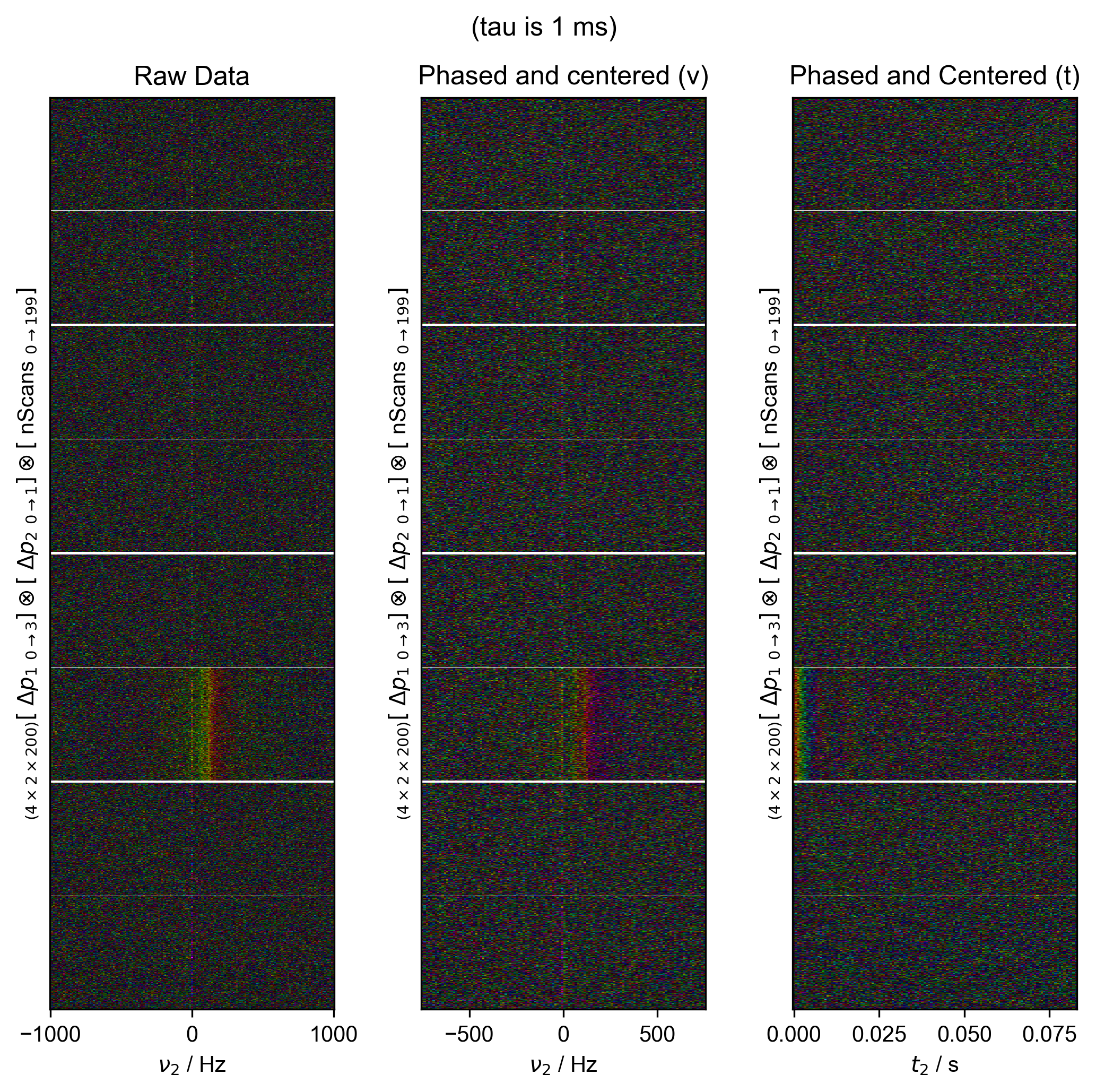
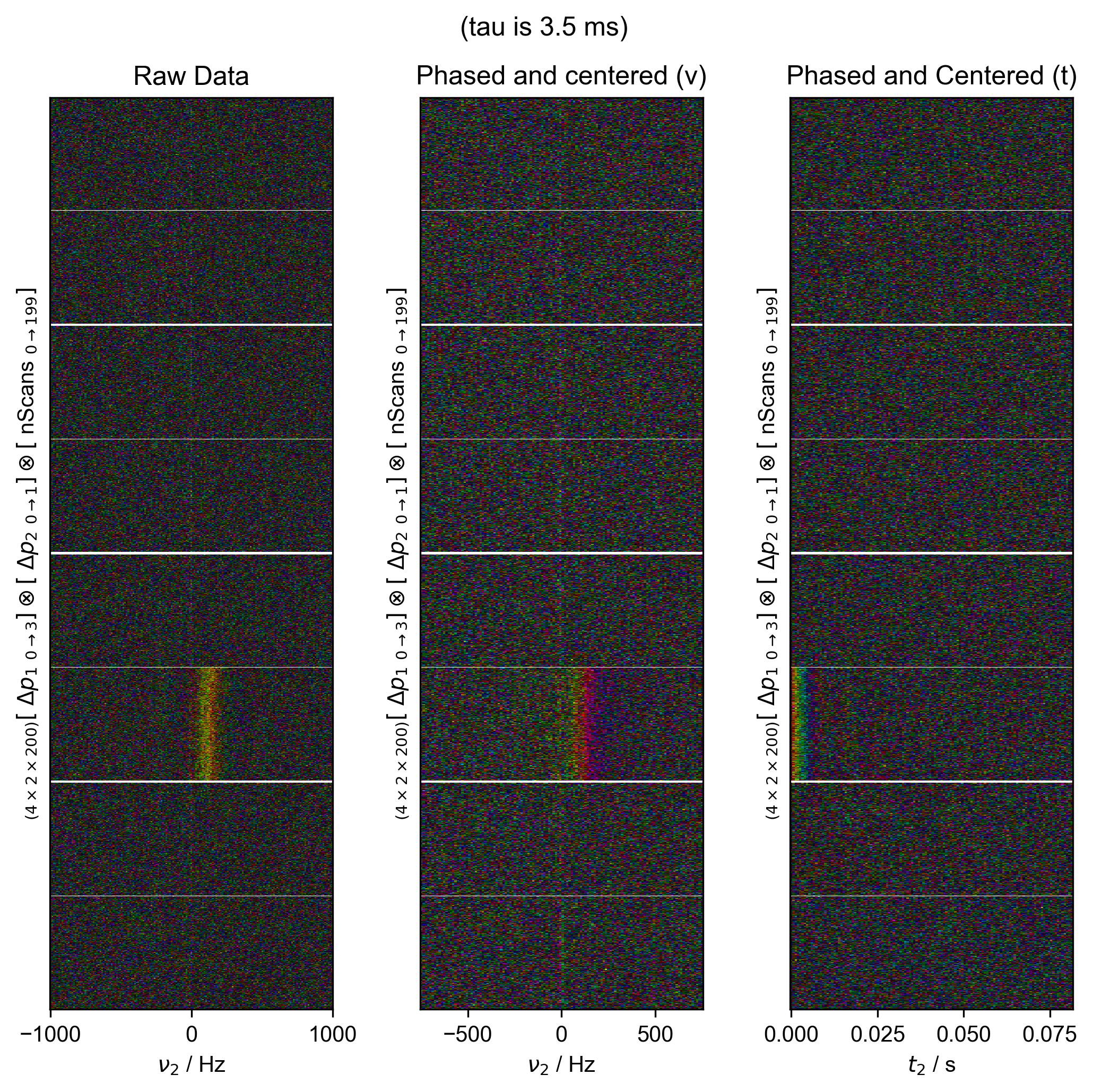
FID from Echo after Phasing and Timing Correction – Challenging Actual Data

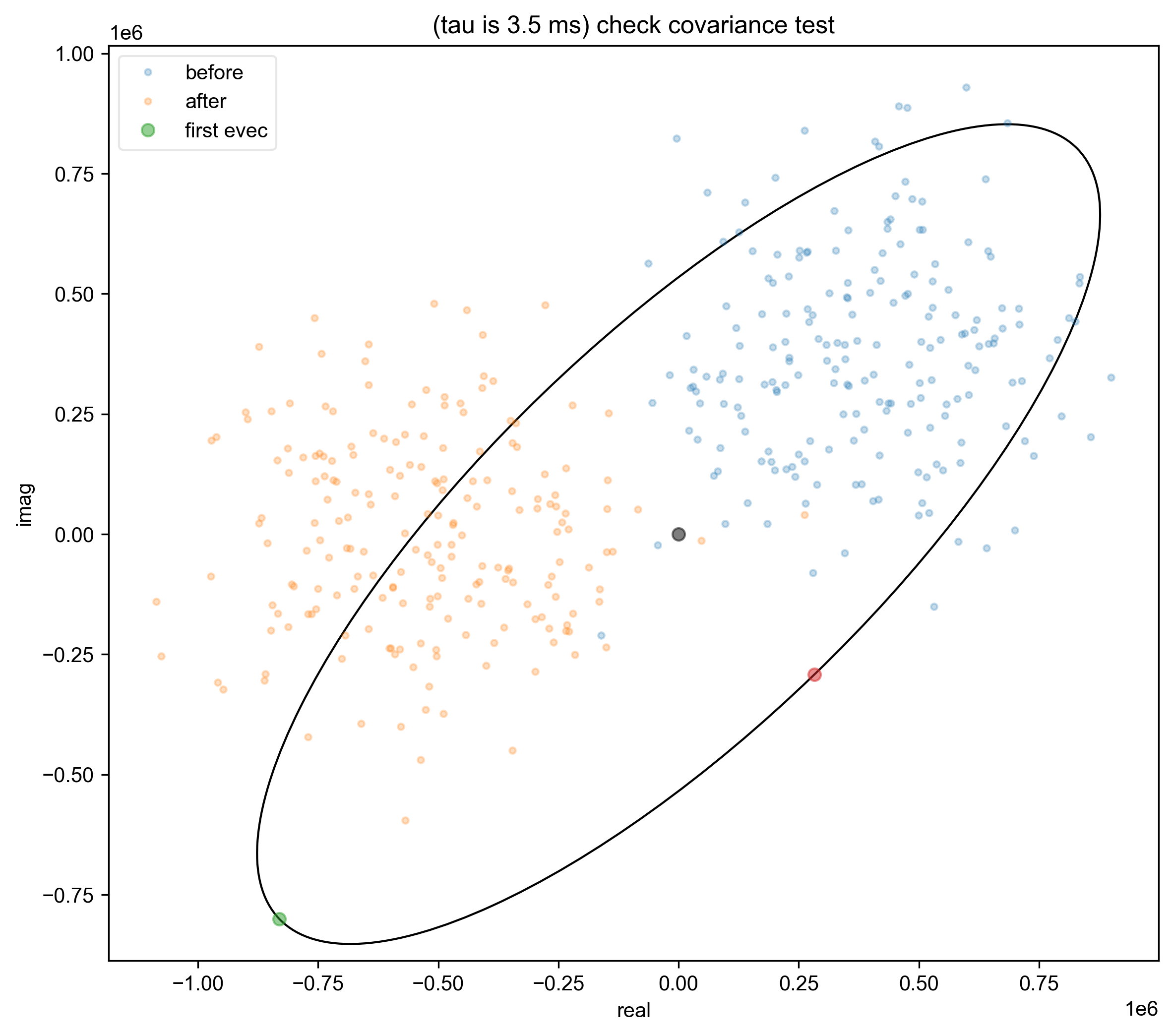
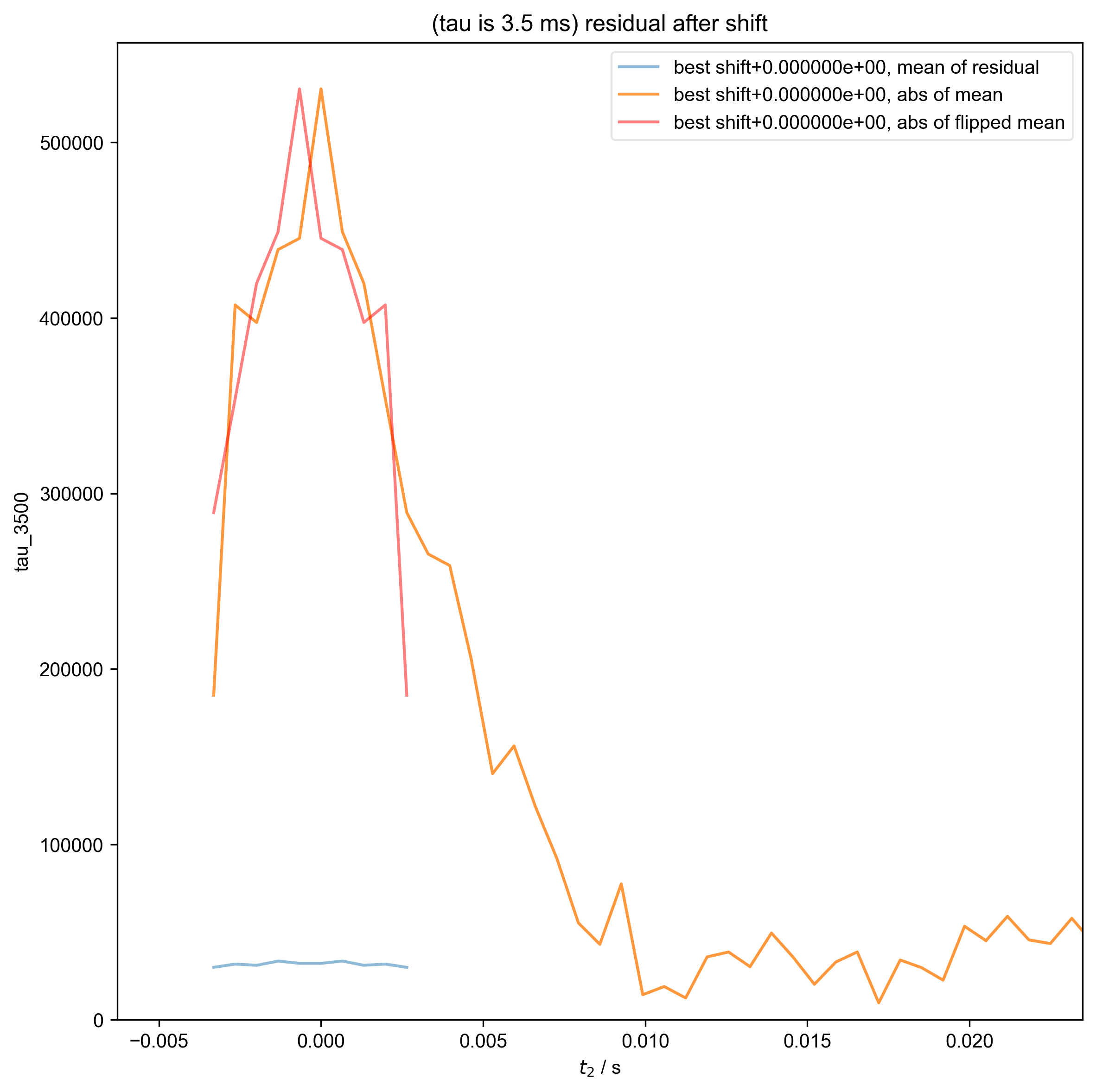
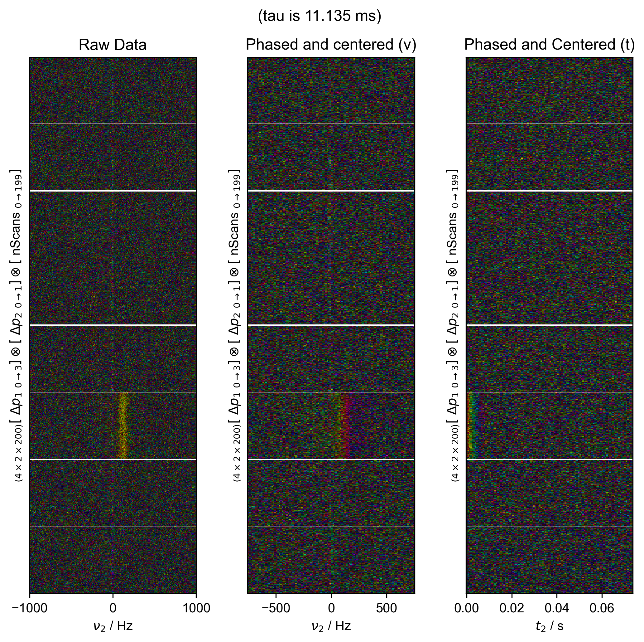
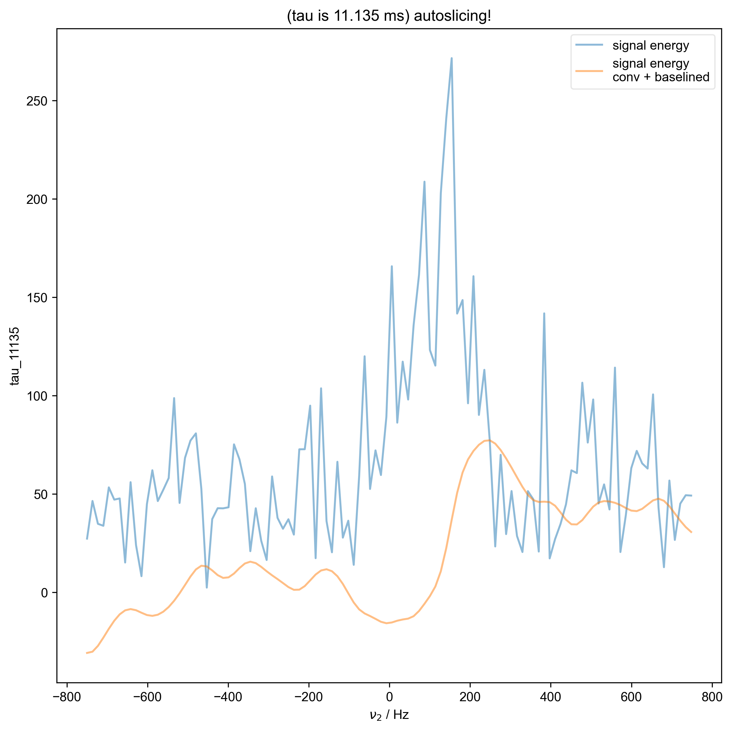
Take real data with varying echo times, and demonstrate how we can automatically find the zeroth order phase and the center of the echo and then slice, in order to get a properly phased FID.

Here we see this

This example provides a challenging test case, with low SNR data (from AOT RMs), one of which has a very short echo time.

• 
• 
• 
• 
• 
• 
• 
• 
• 
• 
• 
• 
• 
• 
• 

----------  logging output to /home/jmfranck/pyspecdata.0.log  ----------
1: (tau is 1 ms) Data processing |||('Hz', None)
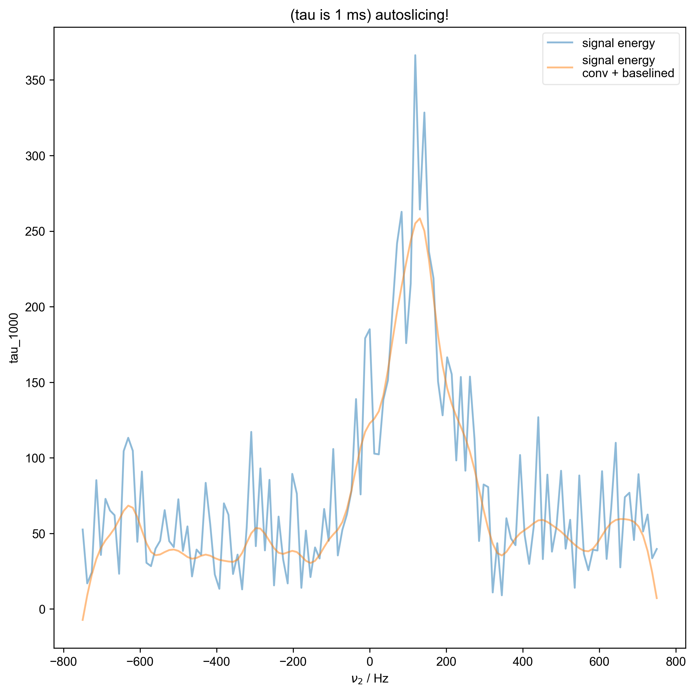
2: (tau is 1 ms) autoslicing!
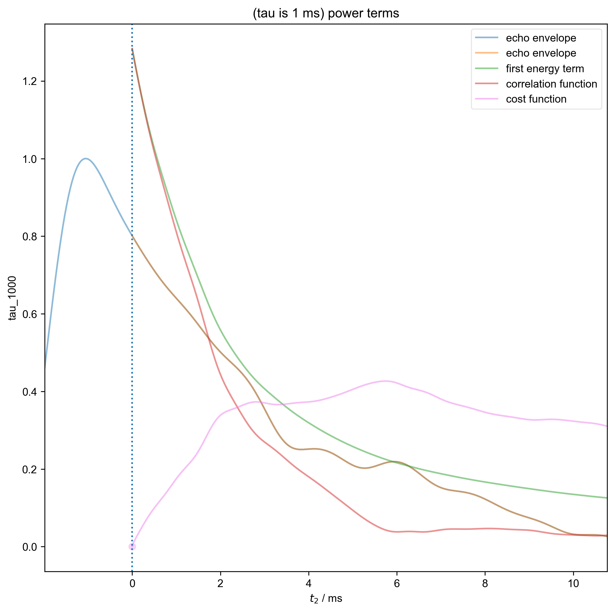
3: (tau is 1 ms) power terms |||ms
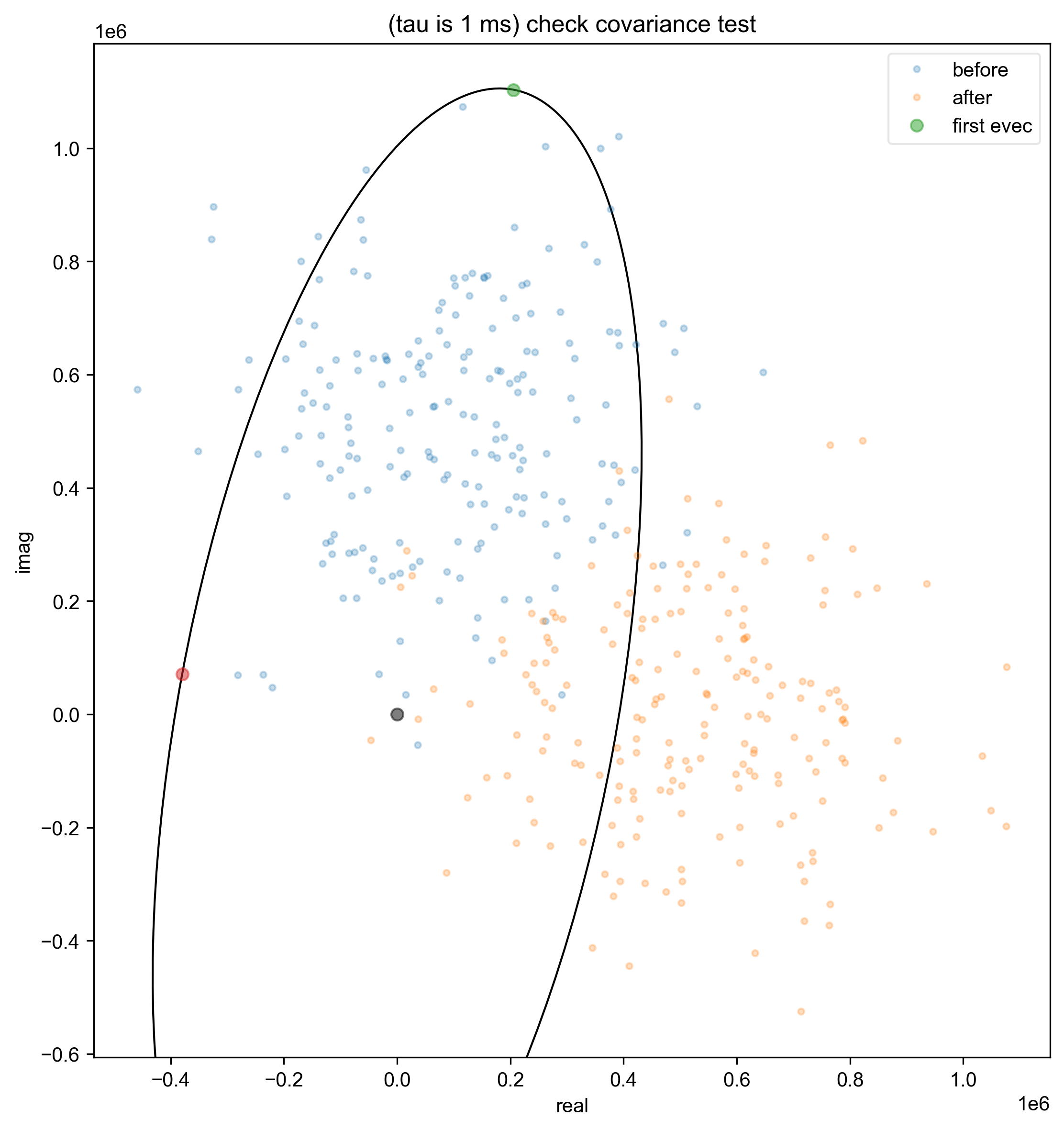
4: (tau is 1 ms) check covariance test
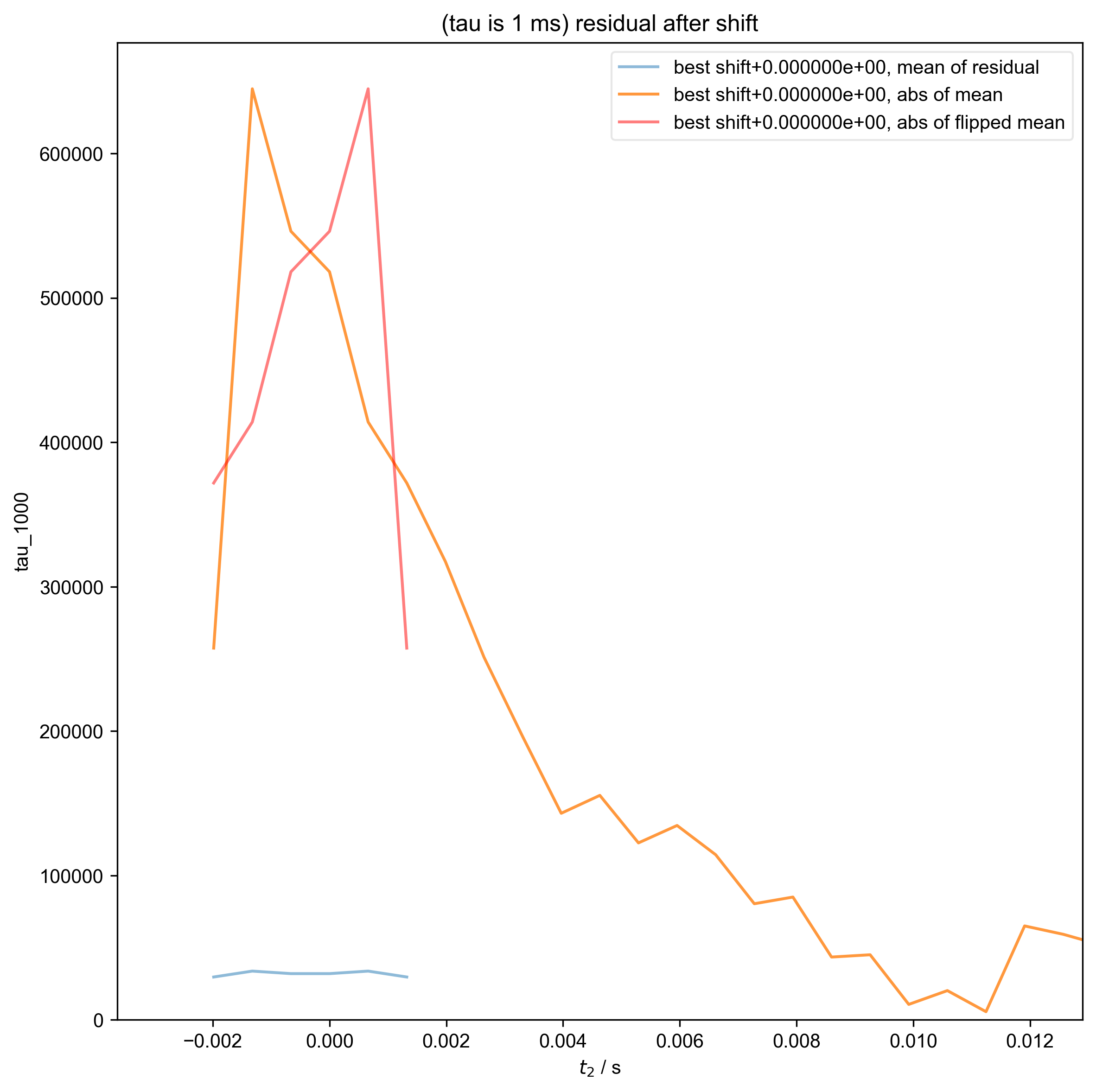
5: (tau is 1 ms) residual after shift
6: (tau is 3.5 ms) Data processing |||('Hz', None)
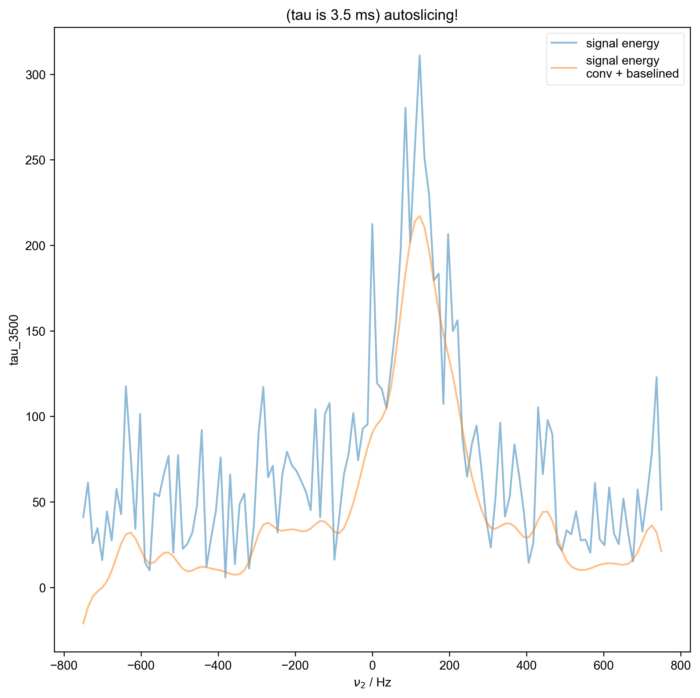
7: (tau is 3.5 ms) autoslicing!
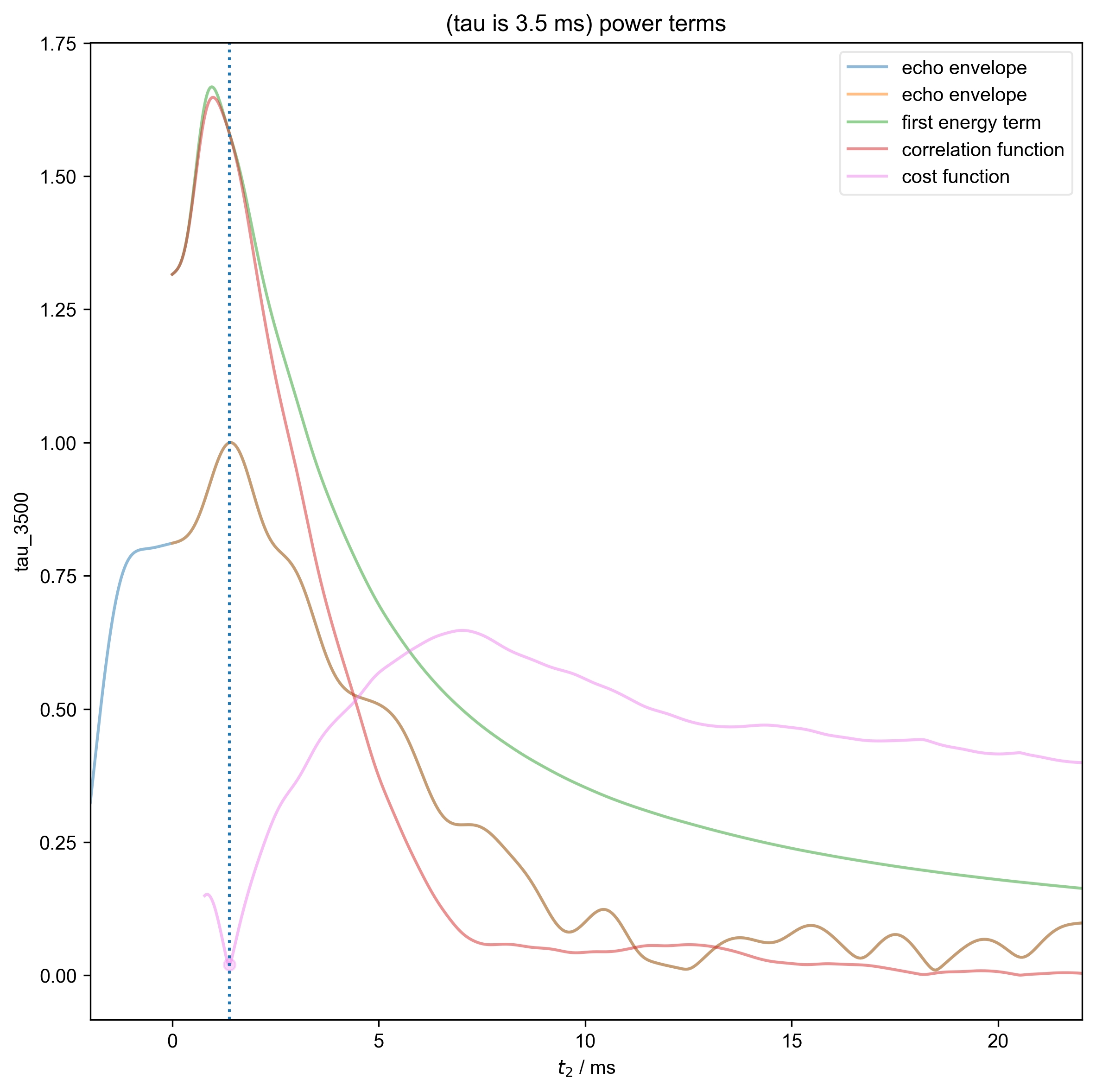
8: (tau is 3.5 ms) power terms |||ms
9: (tau is 3.5 ms) check covariance test
10: (tau is 3.5 ms) residual after shift
11: (tau is 11.135 ms) Data processing |||('Hz', None)
12: (tau is 11.135 ms) autoslicing!
13: (tau is 11.135 ms) power terms |||ms
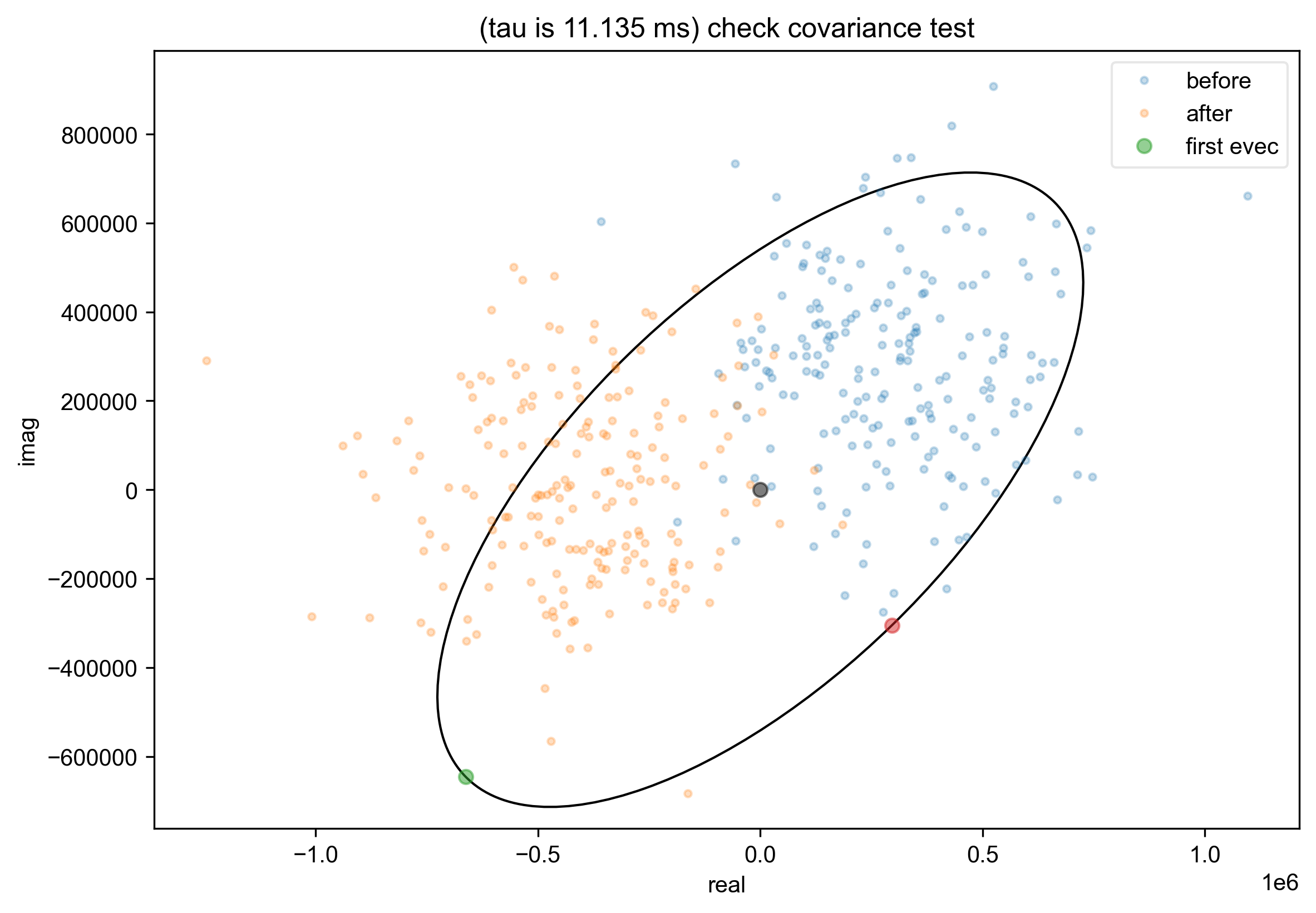
14: (tau is 11.135 ms) check covariance test
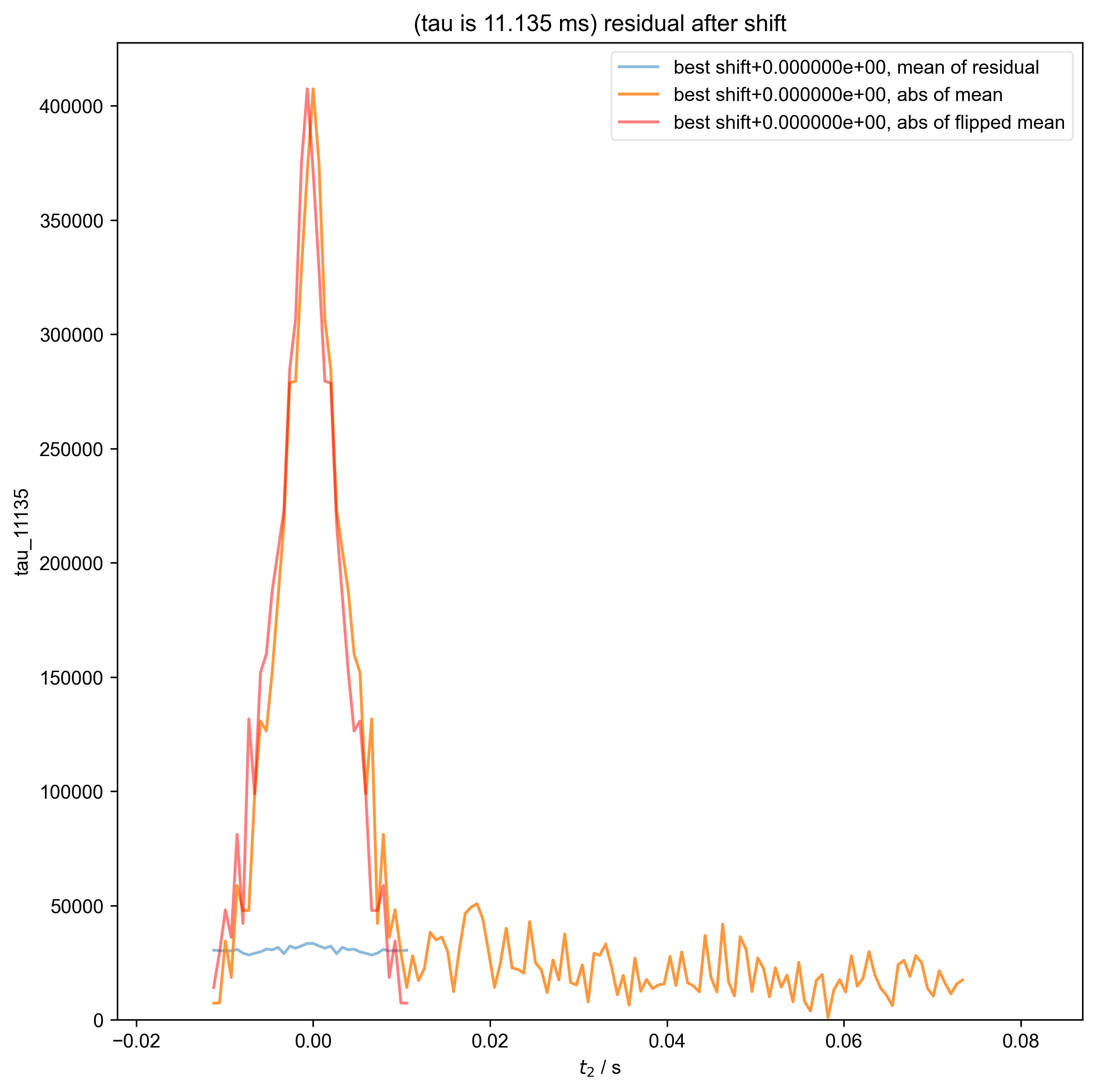
15: (tau is 11.135 ms) residual after shift

from pyspecdata import *
from pyspecProcScripts import *
from pylab import *
import sympy as s
from collections import OrderedDict
from numpy.random import normal
from scipy.signal import tukey

init_logging(level="debug")

rcParams["image.aspect"] = "auto"  # needed for sphinx gallery

# sphinx_gallery_thumbnail_number = 1
t2, td, vd, power, ph1, ph2 = s.symbols("t2 td vd power ph1 ph2")
f_range = (
    -0.75e3,
    0.75e3,
)  # to deal with the shorter echoes, we really just need to use shorter dwell times
filename = "210604_50mM_4AT_AOT_w11_cap_probe_echo"
signal_pathway = {"ph1": 1, "ph2": 0}
with figlist_var() as fl:
    for nodename, file_location, postproc, label, alias_slop in [
        (
            "tau_1000",
            "ODNP_NMR_comp/Echoes",
            "spincore_echo_v1",
            "tau is 1 ms",
            1,
        ),
        (
            "tau_3500",
            "ODNP_NMR_comp/Echoes",
            "spincore_echo_v1",
            "tau is 3.5 ms",
            3,
        ),
        (
            "tau_11135",
            "ODNP_NMR_comp/Echoes",
            "spincore_echo_v1",
            "tau is 11.135 ms",
            3,
        ),
    ]:
        data = find_file(
            filename,
            exp_type=file_location,
            expno=nodename,
            postproc=postproc,
            lookup=lookup_table,
        )
        fl.basename = "(%s)" % label
        fig, ax_list = subplots(1, 3, figsize=(7, 7))
        fig.suptitle(fl.basename)
        data.reorder(["ph1", "ph2", "nScans", "t2"])
        fl.next("Data processing", fig=fig)
        fl.image(data["t2":(-1e3, 1e3)], ax=ax_list[0])
        ax_list[0].set_title("Raw Data")
        data = data["t2":f_range]
        fl.basename = "(%s)" % label
        data = fid_from_echo(data, signal_pathway, fl=fl)
        fl.image(data["t2":(-1e3, 1e3)], ax=ax_list[1], human_units=False)
        ax_list[1].set_title("Phased and centered (ν)")
        data.ift("t2")
        fl.image(data, ax=ax_list[2], human_units=False)
        ax_list[2].set_title("Phased and Centered (t)")
        fig.tight_layout(rect=[0, 0.03, 1, 0.95])