Generate a PSD from SpinCore Data

Here, data containing the noise signal acquired on the SpinCore is converted to a power spectral density and convolved to display a smooth spectra illustrating the noise power.

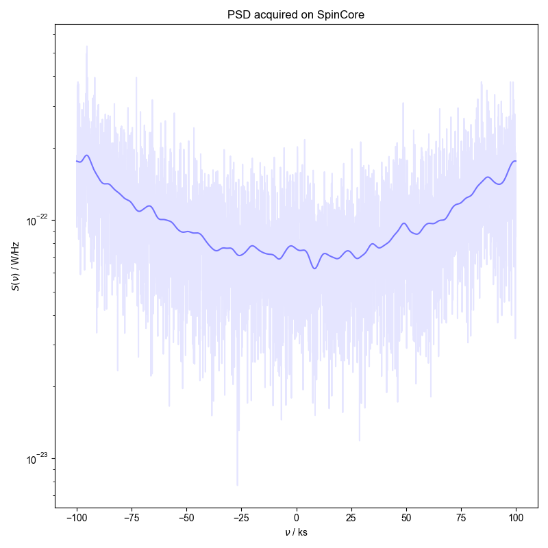
1: PSD acquired on SpinCore |||ks

from numpy import r_
import pyspecdata as psd
from pyspecProcScripts import lookup_table
from pylab import diff, sqrt

lambda_G = 4e3  # Width for Gaussian convolution
dg_per_V = 583e6  # Calibration coefficient to convert the
#                  intrinsic SC units to V at the input of
#                  the receiver. Note this value will change
#                  with different SW
filename = "230822_BNC_RX_magon_200kHz.h5"
with psd.figlist_var() as fl:
    # Load data and apply preprocessing
    s = psd.find_file(
        filename,
        exp_type="ODNP_NMR_comp/Echoes",
        expno="signal",
        postproc="spincore_general",
        lookup=lookup_table,
    )
    s.rename("nScans", "capture")  # To be more consistent
    #                               with the oscilloscope
    #                               data, rename the nScans
    #                               dimension
    s /= dg_per_V  # Convert the intrinsic units of the SC
    #               to $V_{p}$
    s.set_units("t", "s")
    # Calculate $t_{acq}$
    acq_time = diff(s.getaxis("t")[r_[0, -1]])[0]
    s /= sqrt(
        2
    )  # Instantaneous Vₚ√s / √Hz to
    #    Vᵣₘₛ√s / √Hz
    # {{{ equation 21
    s = abs(s) ** 2  # Take mod squared to convert to
    #                   energy $\frac{V_{rms}^{2} \cdot s}{Hz}$
    s.mean("capture")  # Average captures
    s /= acq_time  # Convert to Power $\frac{V_{rms}^2}{Hz} = W$
    s /= 50  # Divide by impedance $\rightarrow$ W/Hz
    # }}}
    # Plot unconvolved PSD on a semilog plot
    s.name(r"$S(\nu)$").set_units("W/Hz")
    fl.next("PSD acquired on SpinCore")
    fl.plot(s, color="blue", alpha=0.1, plottype="semilogy")
    # Convolve using the $\lambda_{G}$ specified above
    s.convolve("t", lambda_G, enforce_causality=False)
    # Plot the convolved PSD on the semilog plot with the
    # unconvolved
    fl.plot(s, color="blue", alpha=0.5, plottype="semilogy")