Check NMR/ESR resonance ratio using a field sweep

Analyzes field sweep data. Determines the optimal field across a gradient that is on-resonance with the Bridge 12 μw frequency stored in the file to determine the resonance ratio of MHz/GHz.

• 
• 
• 
• 
• 

You didn't set units for indirect before saving the data!!!
#d62728
#d62728
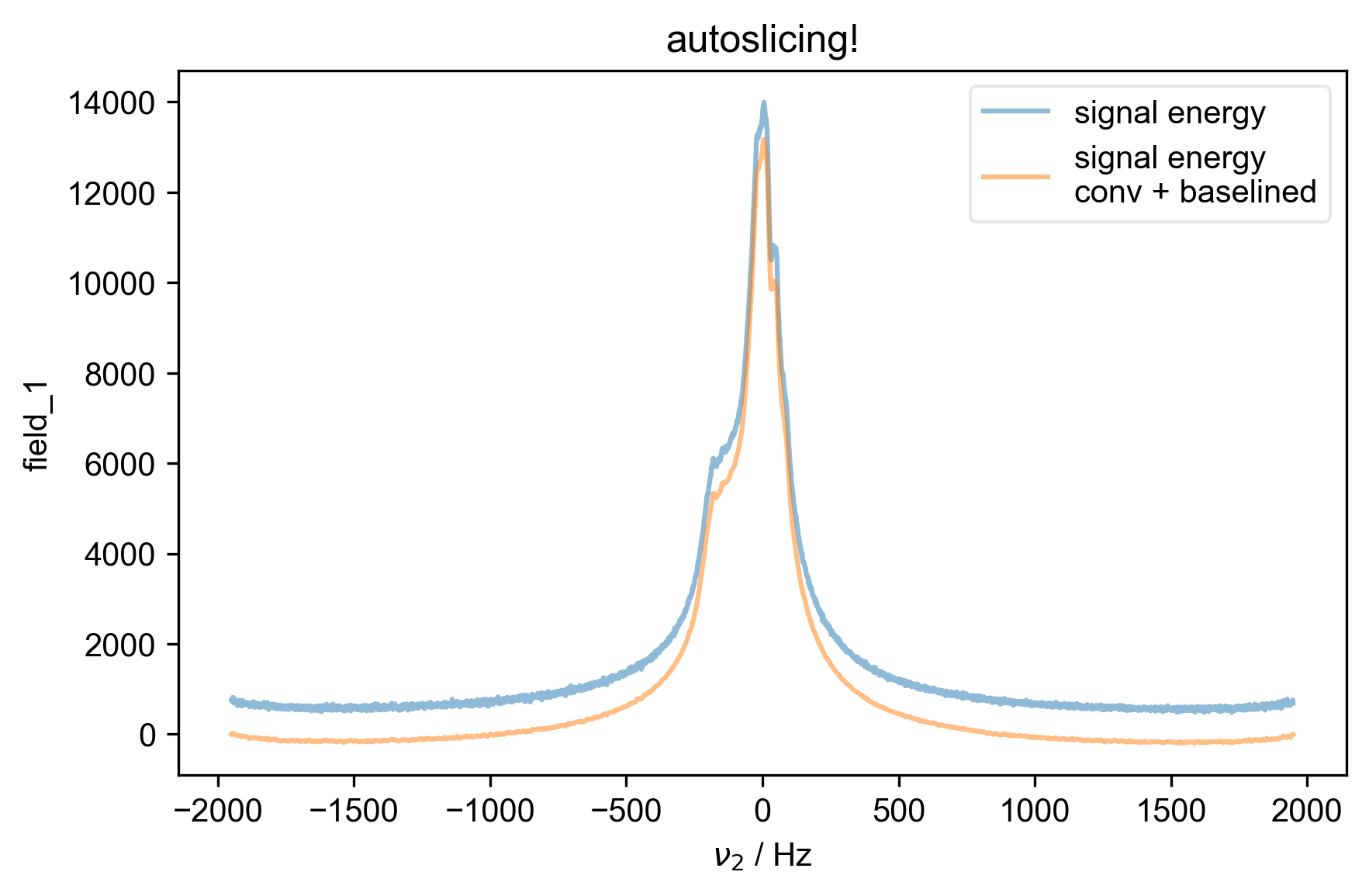
1: autoslicing!
2: Raw Data with averaged scans
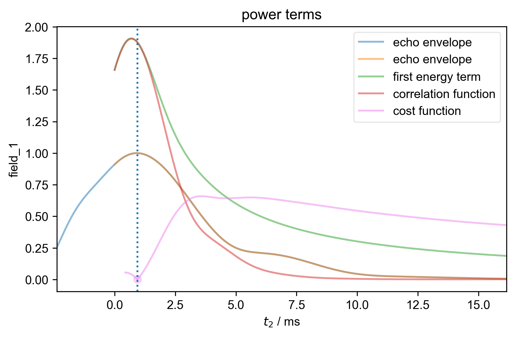
3: power terms |||ms
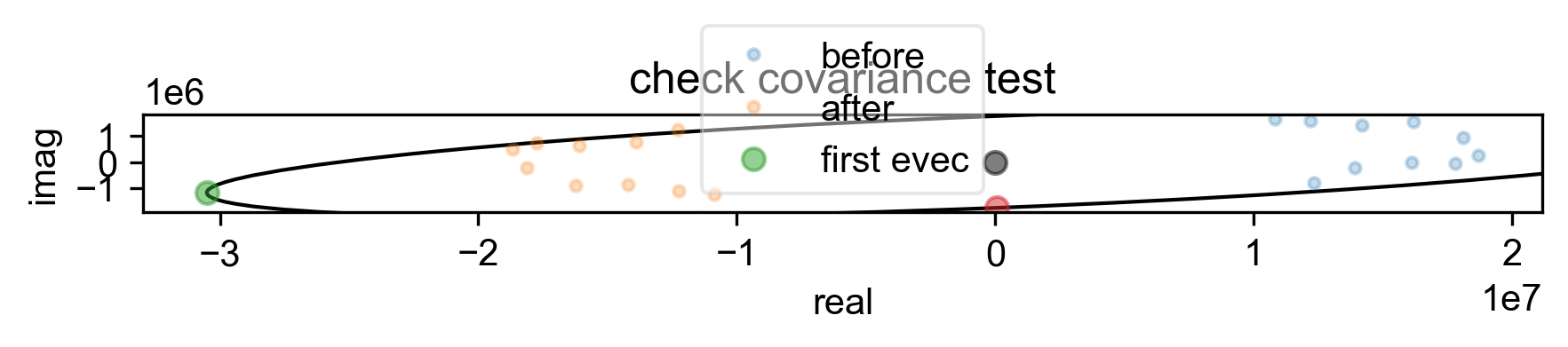
4: check covariance test
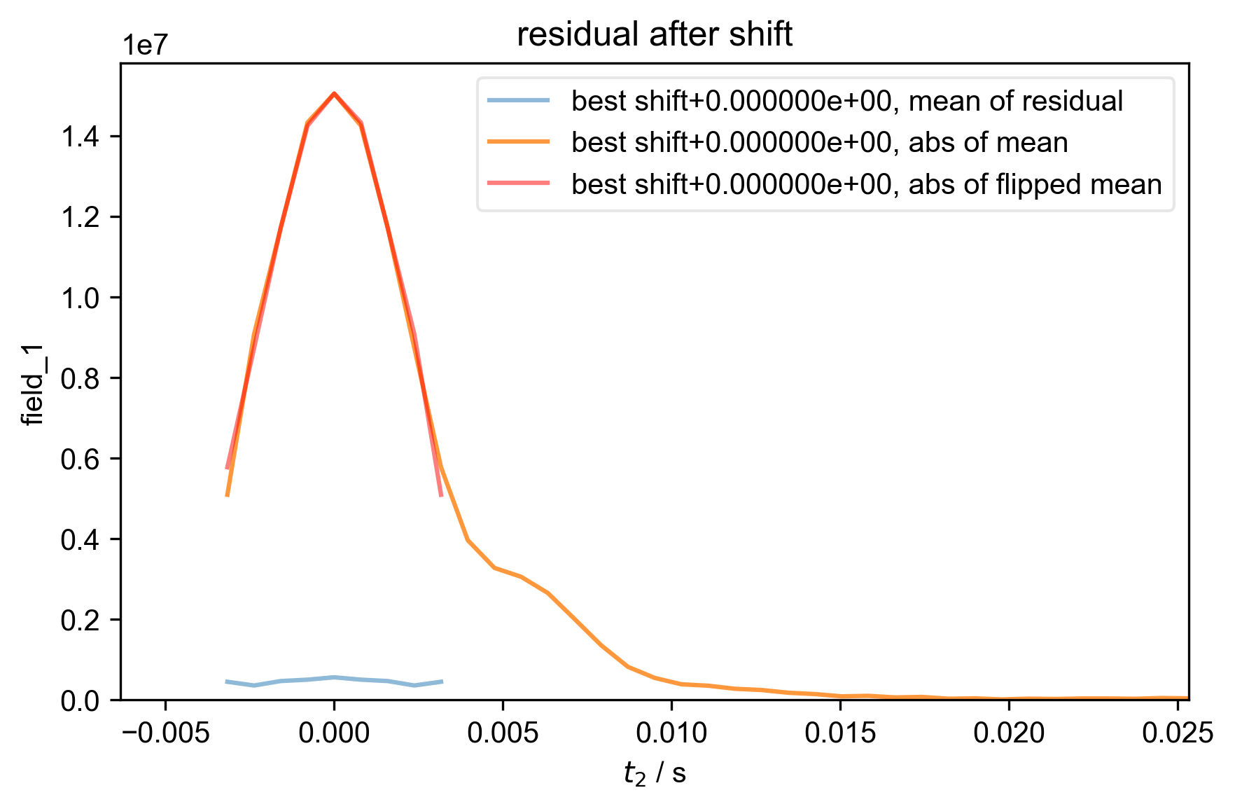
5: residual after shift |||('Hz', 'ppt')

import pyspecdata as psd
import pyspecProcScripts as prscr
import numpy as np
import matplotlib as mpl
import matplotlib.pyplot as plt
from numpy import r_

plt.rcParams["image.aspect"] = "auto"  # needed for sphinx gallery
# sphinx_gallery_thumbnail_number = 2
plt.rcParams.update({
    "errorbar.capsize": 2,
    "figure.facecolor": (1.0, 1.0, 1.0, 0.0),  # clear
    "axes.facecolor": (1.0, 1.0, 1.0, 0.9),  # 90% transparent white
    "savefig.facecolor": (1.0, 1.0, 1.0, 0.0),  # clear
    "savefig.bbox": "tight",
    "savefig.dpi": 300,
    "figure.figsize": (6, 4),
})

thisfile, exp_type, nodename, label_str = (
    "240924_13p5mM_TEMPOL_field.h5",
    "ODNP_NMR_comp/field_dependent",
    "field_1",
    "240924 13.5 mM TEMPOL field sweep",
)
s = psd.find_file(
    thisfile,
    exp_type=exp_type,
    expno=nodename,
    lookup=prscr.lookup_table,
)
use_freq = True
with psd.figlist_var(black=False) as fl:
    nu_B12 = s.get_prop("acq_params")["uw_dip_center_GHz"]
    if use_freq:
        # Unusually, we want to keep the units of the frequency in MHz
        # (rather than Hz), because it makes it easier to calculate the
        # ppt value.
        s["indirect"] = s["indirect"]["carrierFreq"]
        s.set_units("indirect", "MHz")
        s["indirect"] = s["indirect"] / nu_B12
        s.set_units("indirect", "ppt")
    else:
        # if we wanted to plot the field instead, we could set use_freq
        # above to False
        s["indirect"] = s["indirect"]["Field"]
        s.set_units("indirect", "G")
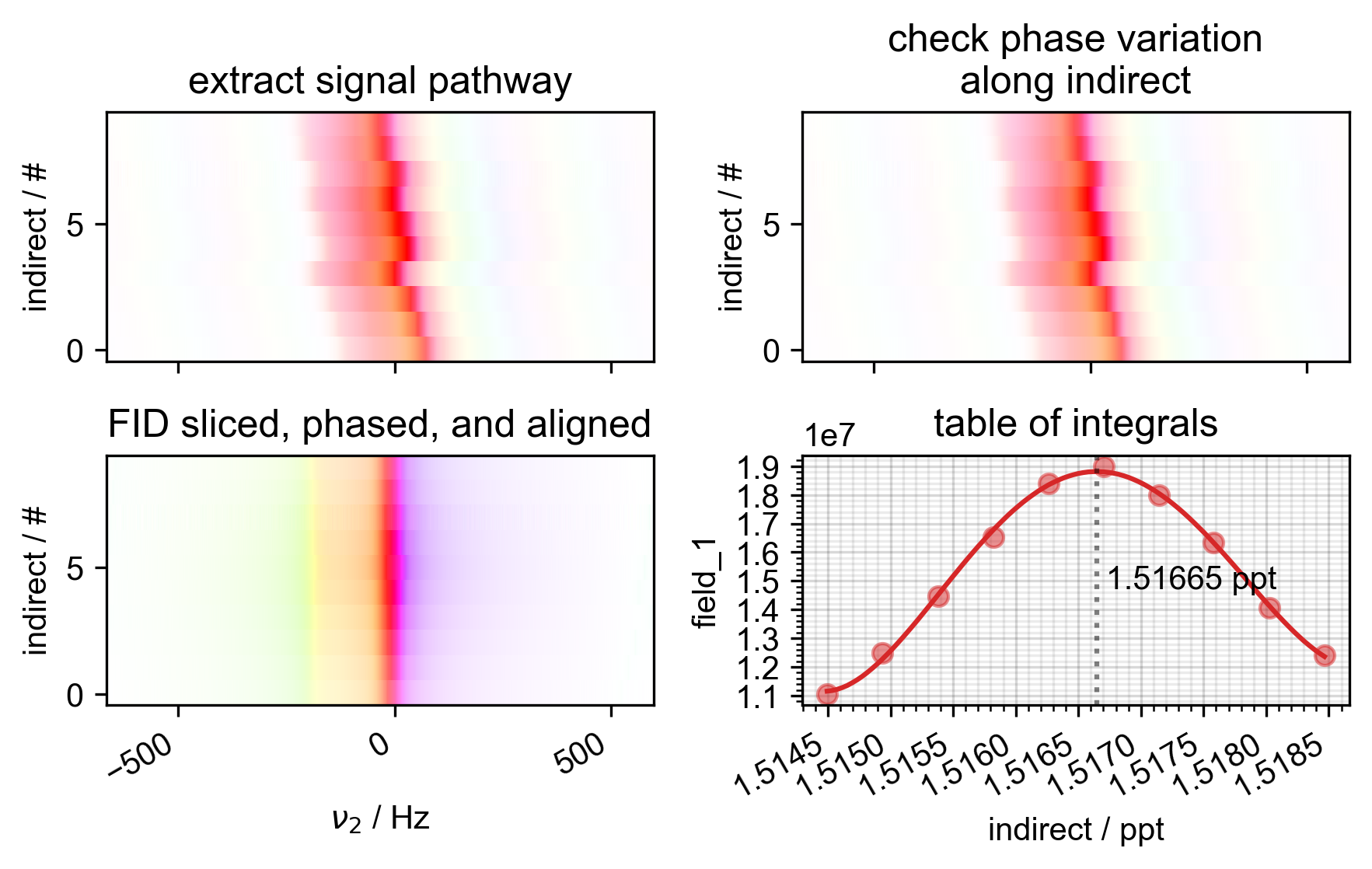
    s, ax4 = prscr.rough_table_of_integrals(s, fl=fl)
    if use_freq:
        assert s.get_units("indirect") == "ppt", "doesn't seem to be in ppt"
        # {{{ use analytic differentiation to find the max of the polynomial
        c_poly = s.polyfit("indirect", 4)
        print(s.get_plot_color())
        forplot = s.eval_poly(c_poly, "indirect", npts=100)
        print(forplot.get_plot_color())
        psd.plot(forplot, label="fit", ax=ax4)
        theroots = np.roots(
            (c_poly[1:] * r_[1 : len(c_poly)])[  # differentiate the polynomial
                ::-1
            ]  # in numpy, poly coeff are backwards
        )
        theroots = theroots[
            np.isclose(theroots.imag, 0)
        ].real  # only real roots
        idx_max = np.argmax(np.polyval(c_poly[::-1], theroots))
        # }}}
        ax4.axvline(x=theroots[idx_max], ls=":", color="k", alpha=0.5)
        ax4.text(
            x=theroots[idx_max],
            y=0.5,
            s=" %0.5f ppt" % theroots[idx_max],
            ha="left",
            va="center",
            color="k",
            transform=mpl.transforms.blended_transform_factory(
                ax4.transData, ax4.transAxes
            ),
        )
    plt.subplots_adjust(hspace=0.5)
    plt.subplots_adjust(wspace=0.3)