Check Integration

Makes sure that automatically chosen integral bounds perform similar to or better than what you would choose by hand.

• 
• 
• 
• 
• 
• 
• 

----------  logging output to /home/jmfranck/pyspecdata.0.log  ----------

from numpy import sqrt, std, r_, pi, exp
from matplotlib.pyplot import rcParams
from pyspecdata import strm, ndshape, nddata, figlist_var, init_logging
from pyspecProcScripts import integral_w_errors
from numpy.random import seed

rcParams["image.aspect"] = "auto"  # needed for sphinx gallery
# sphinx_gallery_thumbnail_number = 2

seed(
    2021
)  # so the same random result is generated every time -- 2021 is meaningless
logger = init_logging(level="debug")
fl = figlist_var()
t2 = nddata(r_[0:1:1024j], "t2")
vd = nddata(r_[0:1:40j], "vd")
ph1 = nddata(r_[0, 2] / 4.0, "ph1")
ph2 = nddata(r_[0:4] / 4.0, "ph2")
signal_pathway = {"ph1": 0, "ph2": 1}
excluded_pathways = [(0, 0), (0, 3)]
manual_slice = (60, 140)  # manually chosen integration bounds
# this generates fake data w/ a T₂ of 0.2s
# amplitude of 21, just to pick a random amplitude
# offset of 300 Hz, FWHM 10 Hz
data = (
    21 * (1 - 2 * exp(-vd / 0.2)) * exp(+1j * 2 * pi * 100 * t2 - t2 * 10 * pi)
)
data *= exp(signal_pathway["ph1"] * 1j * 2 * pi * ph1)
data *= exp(signal_pathway["ph2"] * 1j * 2 * pi * ph2)
data["t2":0] *= 0.5
fake_data_noise_std = 2.0
data.add_noise(fake_data_noise_std)
data.reorder(["ph1", "ph2", "vd"])
# at this point, the fake data has been generated
data.ft(["ph1", "ph2"])
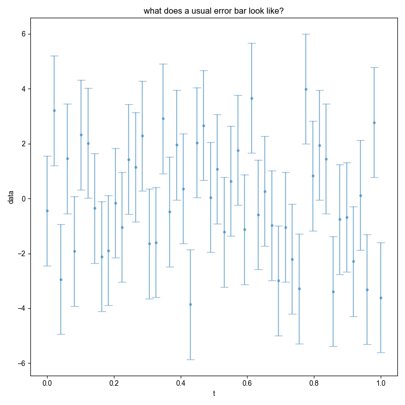
fl.next("what does a usual error bar look like?")
just_noise = nddata(r_[0:1:50j], "t")
just_noise.data *= 0
just_noise.add_noise(fake_data_noise_std)
just_noise.set_error(fake_data_noise_std)
fl.plot(just_noise, ".", capsize=6)
# {{{ usually, we don't use a unitary FT -- this makes it unitary
data /= 0.5 * 0.25  # the dt in the integral for both dims
data /= sqrt(ndshape(data)["ph1"] * ndshape(data)["ph2"])  # normalization
# }}}
data.ft("t2", shift=True)
dt = data.get_ft_prop("t2", "dt")
# {{{ vector-normalize the FT
data /= sqrt(ndshape(data)["t2"]) * dt
# }}}
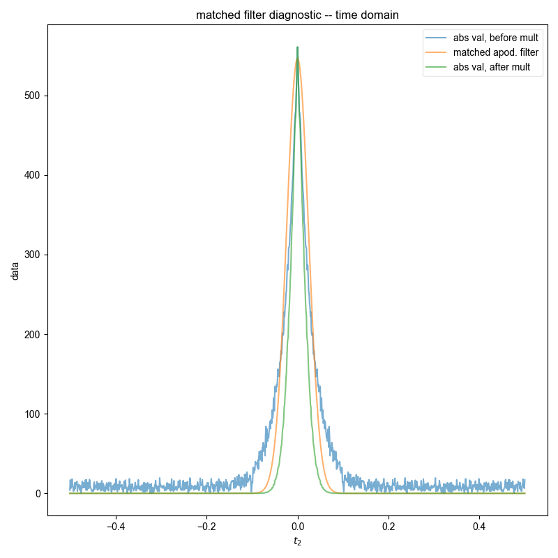
# {{{ First, run the code that automatically chooses integration bounds
# and also assigns error
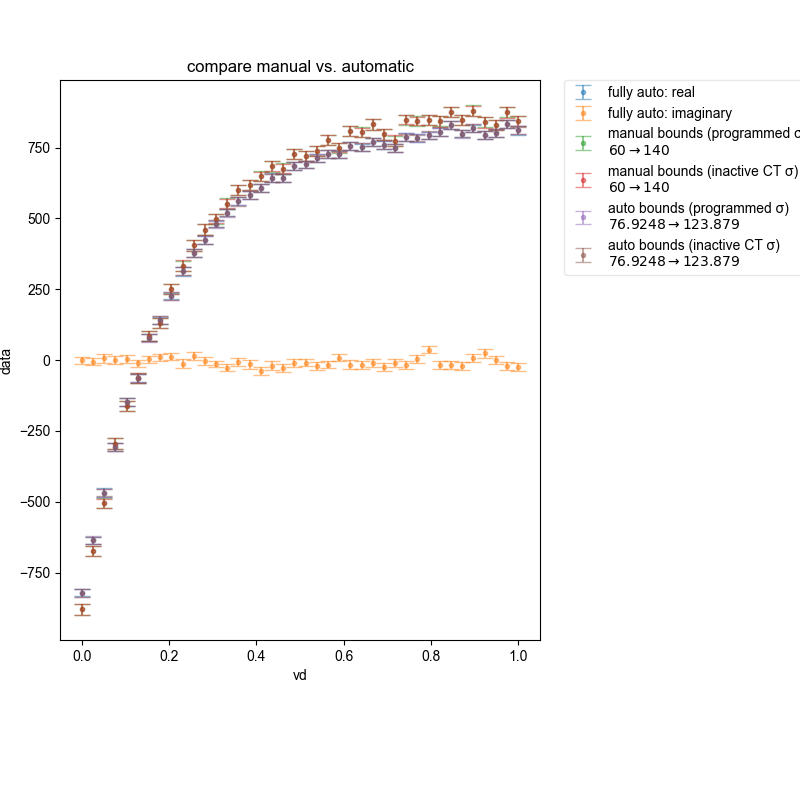
fl.next("compare manual vs. automatic", legend=True)
error_pathway = (
    set(
        (
            (j, k)
            for j in range(ndshape(data)["ph1"])
            for k in range(ndshape(data)["ph2"])
        )
    )
    - set(excluded_pathways)
    - set([(signal_pathway["ph1"], signal_pathway["ph2"])])
)
error_pathway = [{"ph1": j, "ph2": k} for j, k in error_pathway]
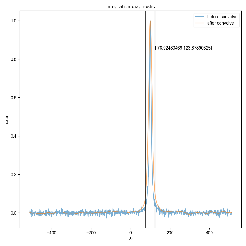
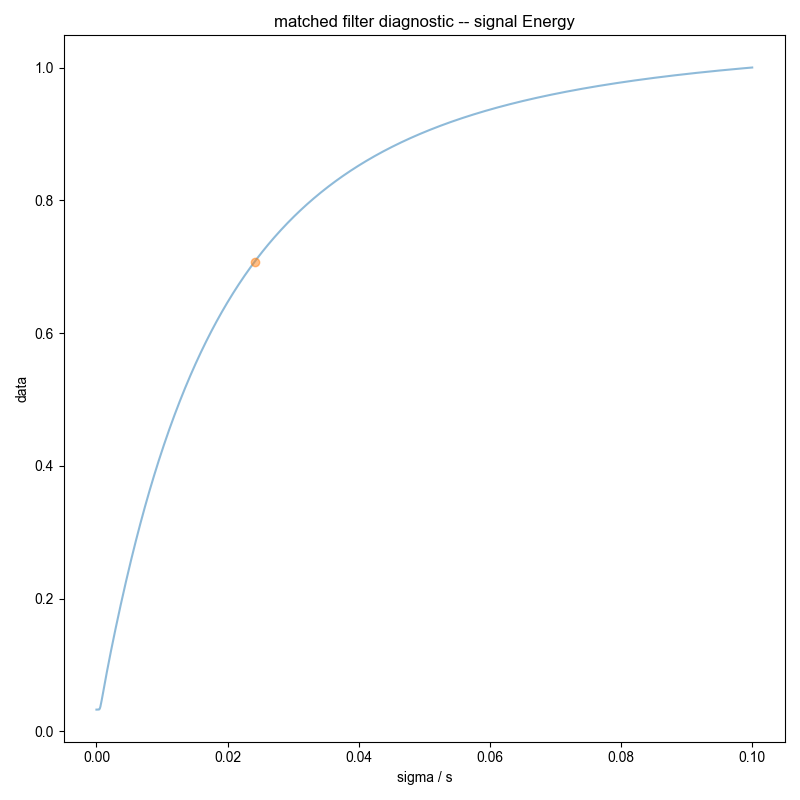
s_int, returned_frq_slice = integral_w_errors(
    data, signal_pathway, error_pathway, fl=fl, return_frq_slice=True
)
fl.plot(s_int, ".", label="fully auto: real", capsize=6)
fl.plot(s_int.imag, ".", label="fully auto: imaginary", capsize=6)
# }}}
logger.debug(
    strm("check the std after FT", std(data["ph1", 0]["ph2", 0].data.real))
)
# the sqrt on the next line accounts for the var(real)+var(imag)
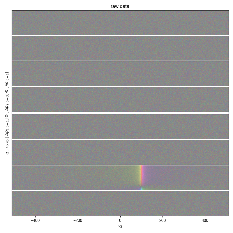
fl.next("raw data")
fl.image(data, alpha=0.5)
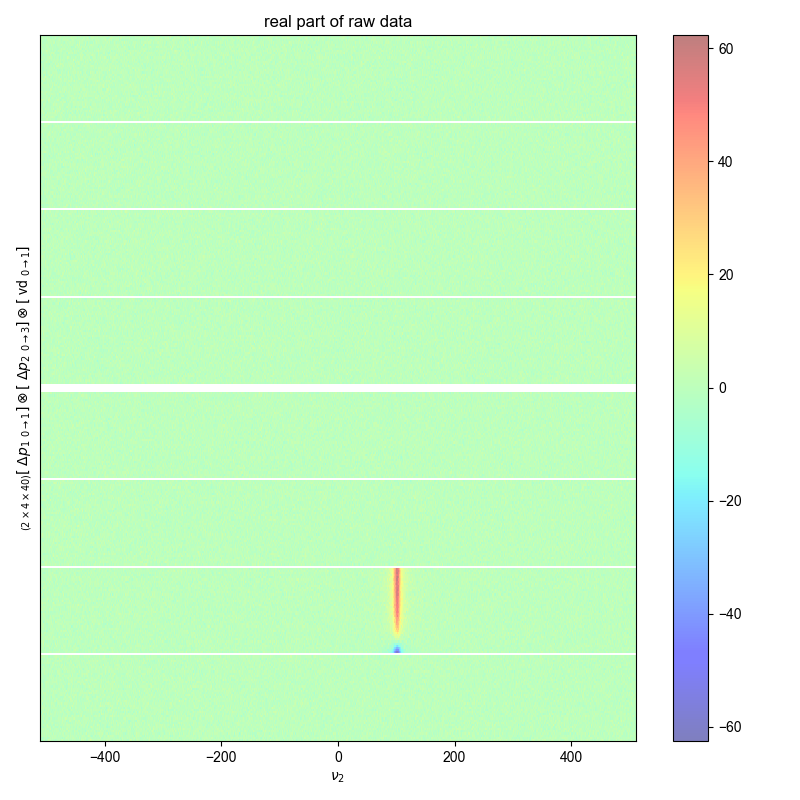
fl.next("real part of raw data")
fl.image(data.real, alpha=0.5)
fl.next("compare manual vs. automatic")
# run a controlled comparison between manually chosen integration bounds and
# compare against automatically generated
# as noted in issue #44 , manually chosen bounds underperform
for bounds, thislabel in [
    (
        manual_slice,
        "manual bounds",
    ),  # leave this as a loop so user can experiment with different bounds
    (
        tuple(returned_frq_slice),
        "auto bounds",
    ),  # leave this as a loop so user can experiment with different bounds
]:
    manual_bounds = data["ph1", 0]["ph2", 1]["t2":bounds]
    assert manual_bounds.get_ft_prop("t2")
    std_from_00 = (
        data["ph1", 0]["ph2", 0]["t2":bounds]
        .C.run(lambda x: abs(x) ** 2 / 2)
        .mean_all_but(["t2", "vd"])
        .mean("t2")
        .run(sqrt)
    )
    logger.debug(
        strm(
            "here is the std calculated from an off pathway",
            std_from_00,
            "does it match",
            fake_data_noise_std,
            "?",
        )
    )
    N = ndshape(manual_bounds)["t2"]
    df = manual_bounds.get_ft_prop("t2", "df")
    logger.debug(
        strm(ndshape(manual_bounds), "df is", df, "N is", N, "N*df is", N * df)
    )
    manual_bounds.integrate("t2")
    # N terms that have variance given by fake_data_noise_std**2 each
    # multiplied by df
    # the 2 has to do w/ real/imag/abs -- see check_integration_error
    propagated_variance = N * df**2 * fake_data_noise_std**2
    propagated_variance_from_inactive = N * df**2 * std_from_00**2
    logger.debug(
        strm(
            "manually calculated integral error is", sqrt(propagated_variance)
        )
    )
    manual_bounds.set_error(sqrt(propagated_variance))
    fl.plot(
        manual_bounds,
        ".",
        capsize=6,
        label="%s (programmed σ)\n$%4g\\rightarrow%4g$"
        % ((thislabel,) + bounds),
        alpha=0.5,
    )
    manual_bounds.set_error(sqrt(propagated_variance_from_inactive.data))
    fl.plot(
        manual_bounds,
        ".",
        capsize=6,
        label="%s (inactive CT σ)\n$%4g\\rightarrow%4g$"
        % ((thislabel,) + bounds),
        alpha=0.5,
    )
fl.show()