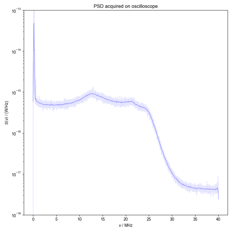
Generate a PSD from Oscilloscope Data

Here, data containing the noise signal acquired on the oscilloscope is converted to a power spectral density and convolved to display a smooth spectra illustrating the noise power.

You didn't set units for capture before saving the data!!!
1: PSD acquired on oscilloscope |||MHz

from numpy import r_
from pyspecdata import figlist_var, find_file
from pylab import diff, sqrt, ylim, ylabel
import re

lambda_G = 0.1e6  # Width for Gaussian convolution
filename = "240328_RX_GDS_2mV_analytic.h5"
nodename = "accumulated_240328"
with figlist_var() as fl:
    # Load data according to the filename and nodename
    s = find_file(
        re.escape(filename),
        expno=nodename,
        exp_type="ODNP_NMR_comp/noise_tests",
    )
    # Calculate $t_{acq}$
    acq_time = diff(s.getaxis("t")[r_[0, -1]])[0]
    s.ft("t")  # V_p√s/√Hz
    # Instantaneous V_p*√s/√Hz -> V_rms√s/√Hz
    s /= sqrt(2)
    # {{{ equation 21
    s = abs(s) ** 2  # Take mod squared to convert to energy
    #                  V_rms^2 s/Hz
    s.mean("capture")  # Average over all captures
    s /= acq_time  # Convert to power V_rms^2/Hz = W
    s /= 50  # Divide by impedance -> W/Hz
    # }}}
    s.set_units("t", "Hz")
    # Plot unconvolved PSD on a semilog plot
    fl.next("PSD acquired on oscilloscope")
    fl.plot(
        s["t":(0, 49e6)],
        color="blue",
        alpha=0.1,
        plottype="semilogy",
    )
    # Convolve using the lambda_G specified above
    s.convolve("t", lambda_G, enforce_causality=False)
    # Plot the convolved PSD on the semilog plot with the unconvolved
    fl.plot(
        s["t":(0, 49e6)],
        color="blue",
        alpha=0.3,
        plottype="semilogy",
    )
    ylim(1e-18, 1e-13)  # set y limits
    ylabel(r"$S(\nu)$ / (W/Hz)")