Captured Nutation

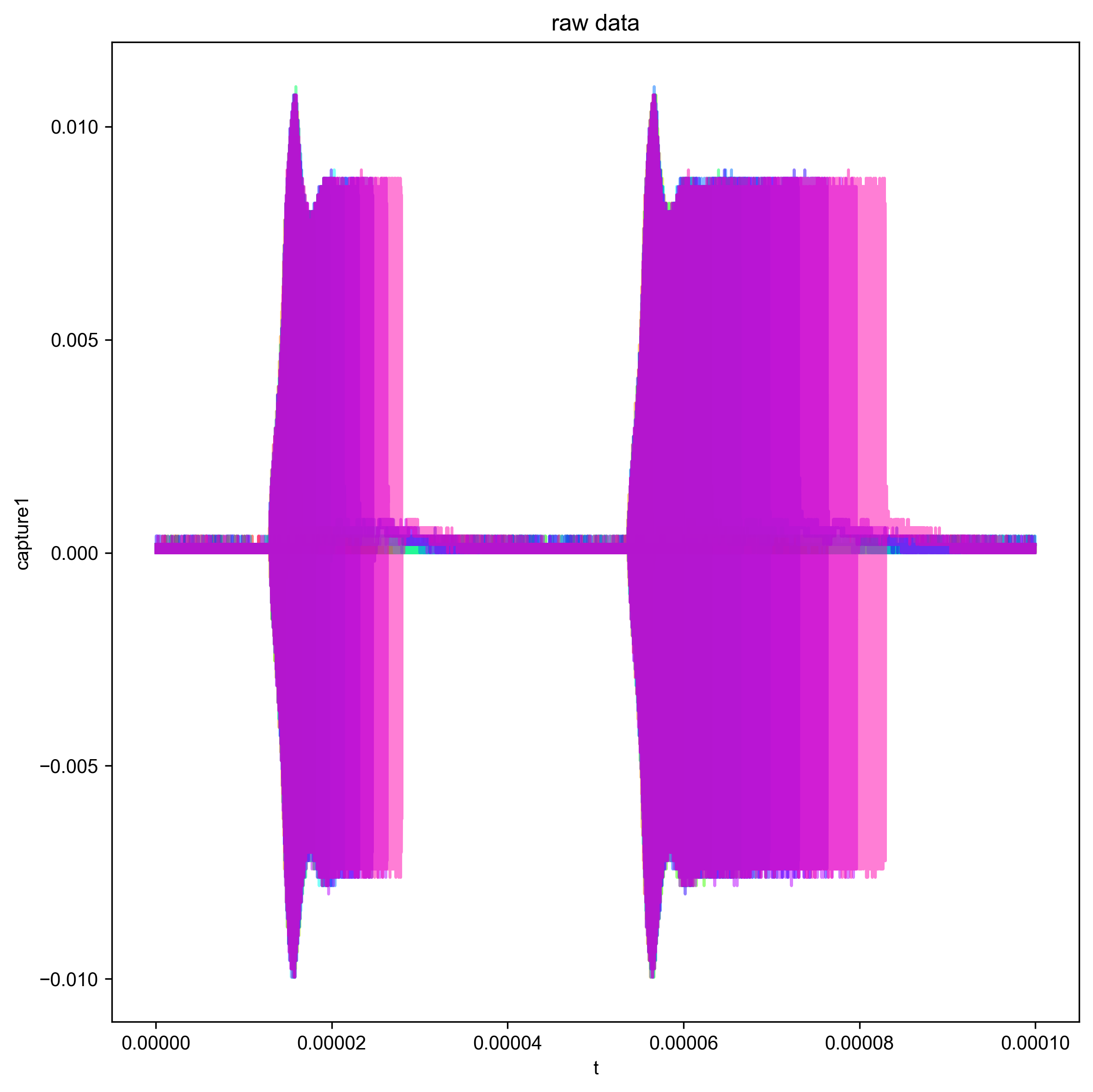
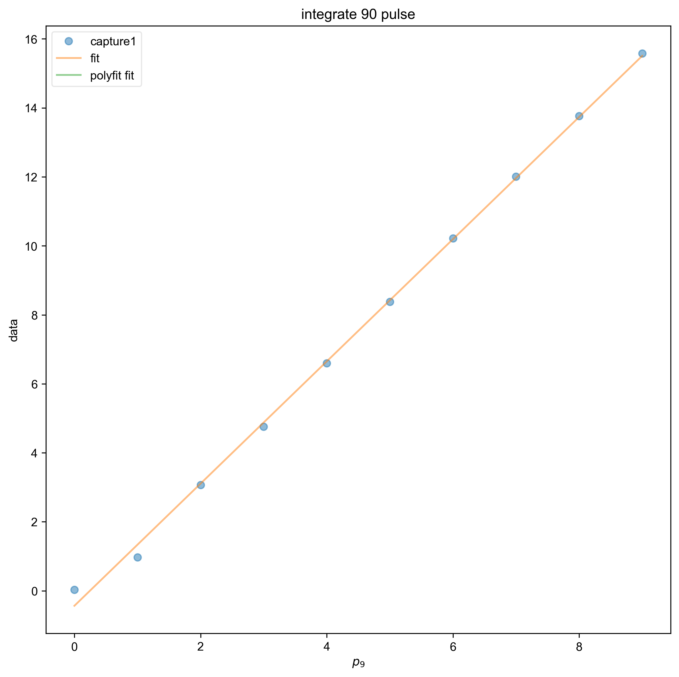
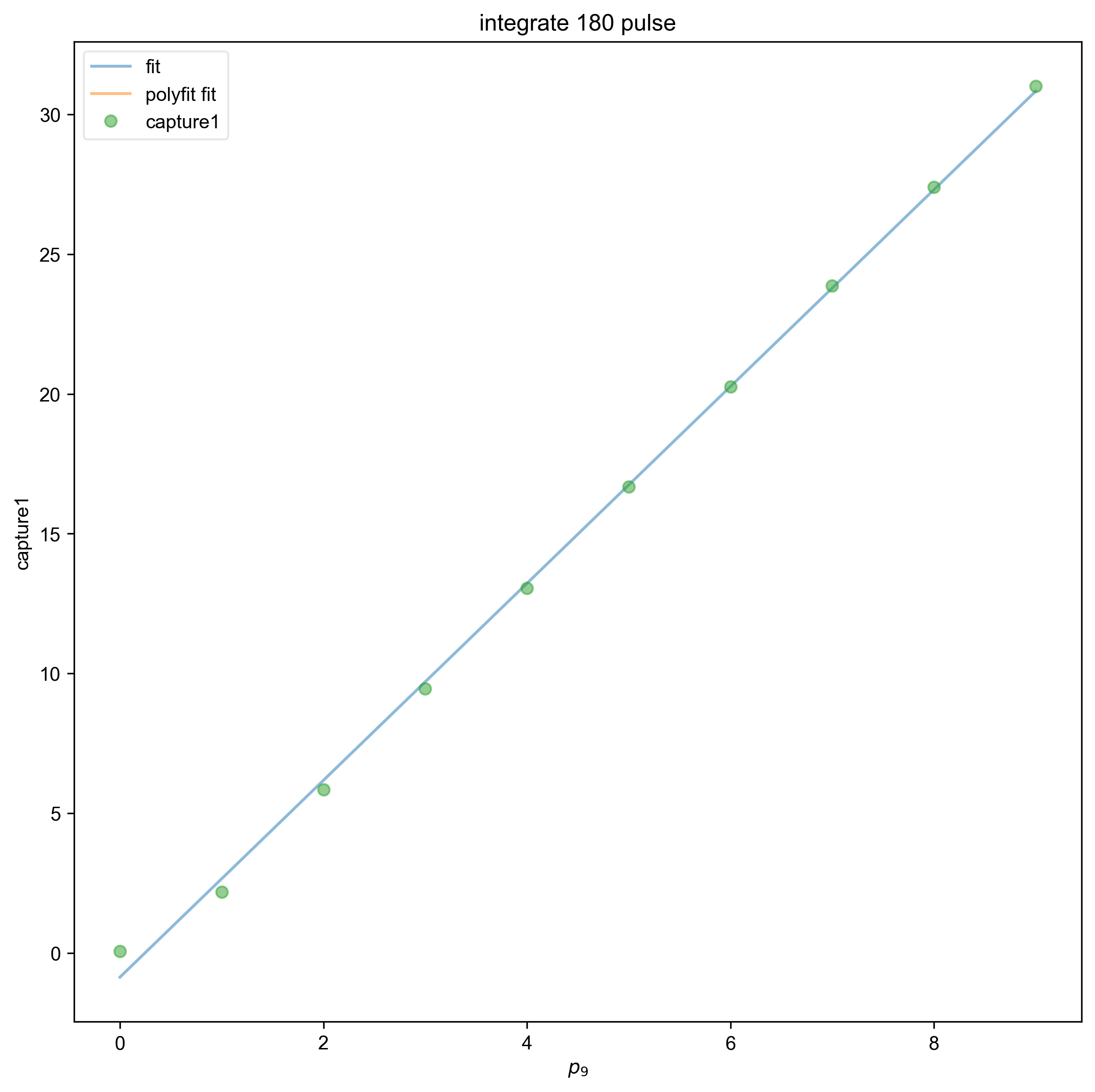
Processes and visualizes the nutation pulse program that has been captured on a oscilloscope. Integrates the 90 and 180 pulse to show linearity.

• 
• 
• 
• 
• 

You didn't set units for p90 before saving the data!!!
You didn't set units for t before saving the data!!!
{\bf Warning:} You have no error associated with your plot, and I want to flag this for now


{\bf Warning:} You have no error associated with your plot, and I want to flag this for now


1: raw data |||(None, None)
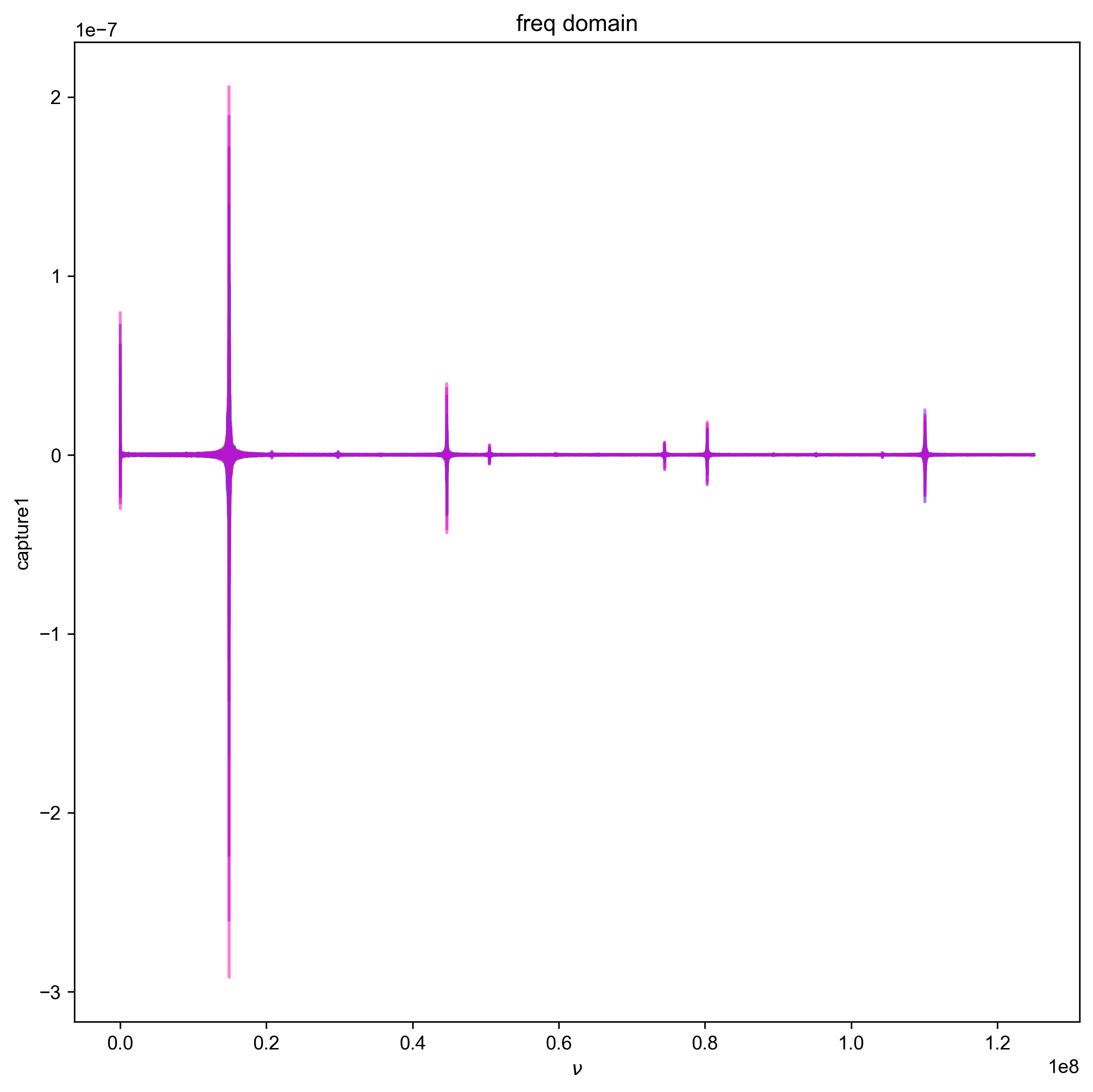
2: freq domain |||(None, None)
3: analytic signal |||None
4: integrate 90 pulse |||None
5: integrate 180 pulse |||None

from pyspecdata import *
from pylab import *
from sympy import symbols, latex, Symbol

rcParams["image.aspect"] = "auto"  # needed for sphinx gallery
# sphinx_gallery_thumbnail_number = 3

with figlist_var() as fl:
    for (
        filename,
        folder_name,
        nodename,
        t_min,
        t_max,
        ninety_range,
        oneeighty_range,
    ) in [
        (
            "210204_gds_p90_vary_3",
            "nutation",
            "capture1",
            1.4e7,
            1.6e7,
            (1.237e-5, 3.09e-5),
            (5.311e-5, 8.8e-5),
        )
    ]:
        d = find_file(filename, exp_type=folder_name, expno=nodename)
        fl.next("raw data")
        fl.plot(d)
        d.ft("t", shift=True)
        d = d["t":(0, None)]  # toss negative frequencies
        #                    multiply data by 2 because the equation
        #                    1/2a*exp(iwt)+aexp(-iwt) and the 2 negated the
        #                    half. taken from analyze_square_refl.py
        d *= 2
        fl.next("freq domain")
        fl.plot(d)
        d["t":(None, t_min)] = 0
        d["t":(t_max, None)] = 0
        d.ift("t")
        fl.next("analytic signal")
        # {{{ plotting abs
        # took out for loop and hard coding p90 times because only GDS parameters saved over
        # the pp parameters
        for j in range(len(d.getaxis("p90"))):
            fl.plot(abs(d["p90", j]), alpha=0.5, linewidth=1)
        # }}}
        d = abs(d)
        # {{{integrating 90 pulse and fitting to line
        ninety_pulse = d["t":ninety_range]
        ninety_pulse = ninety_pulse.sum("t")
        fl.next("integrate 90 pulse")
        line1, fit1 = ninety_pulse.polyfit(
            "p90", order=1, force_y_intercept=None
        )
        fl.plot(ninety_pulse, "o")
        f1 = fitdata(ninety_pulse)
        m, b, p90 = symbols("m b p90", real=True)
        f1.functional_form = m * p90 + b
        f1.fit()
        logger.info(strm("output:", f1.output()))
        logger.info(strm("latex:", f1.latex()))
        fl.plot(f1.eval(100), label="fit")
        fl.plot(fit1, label="polyfit fit")
        logger.info(strm("polyfit for 90 pulse output", line1))
        # }}}
        # {{{integrating 180 pulse and fitting to line
        one_eightypulse = d["t":oneeighty_range]
        one_eightypulse = one_eightypulse.sum("t")
        fl.next("integrate 180 pulse")
        line2, fit2 = one_eightypulse.polyfit(
            "p90", order=1, force_y_intercept=None
        )
        f2 = fitdata(one_eightypulse)
        m, b, p90 = symbols("m b p90", real=True)
        f2.functional_form = m * p90 + b
        f2.fit()
        logger.info(strm("output:", f2.output()))
        logger.info(strm("latex:", f2.latex()))
        fl.plot(f2.eval(100), label="fit")
        logger.info(strm("polyfit for 180 pulse:", line2))
        fl.plot(fit2, label="polyfit fit")
        fl.plot(one_eightypulse, "o")
        # }}}