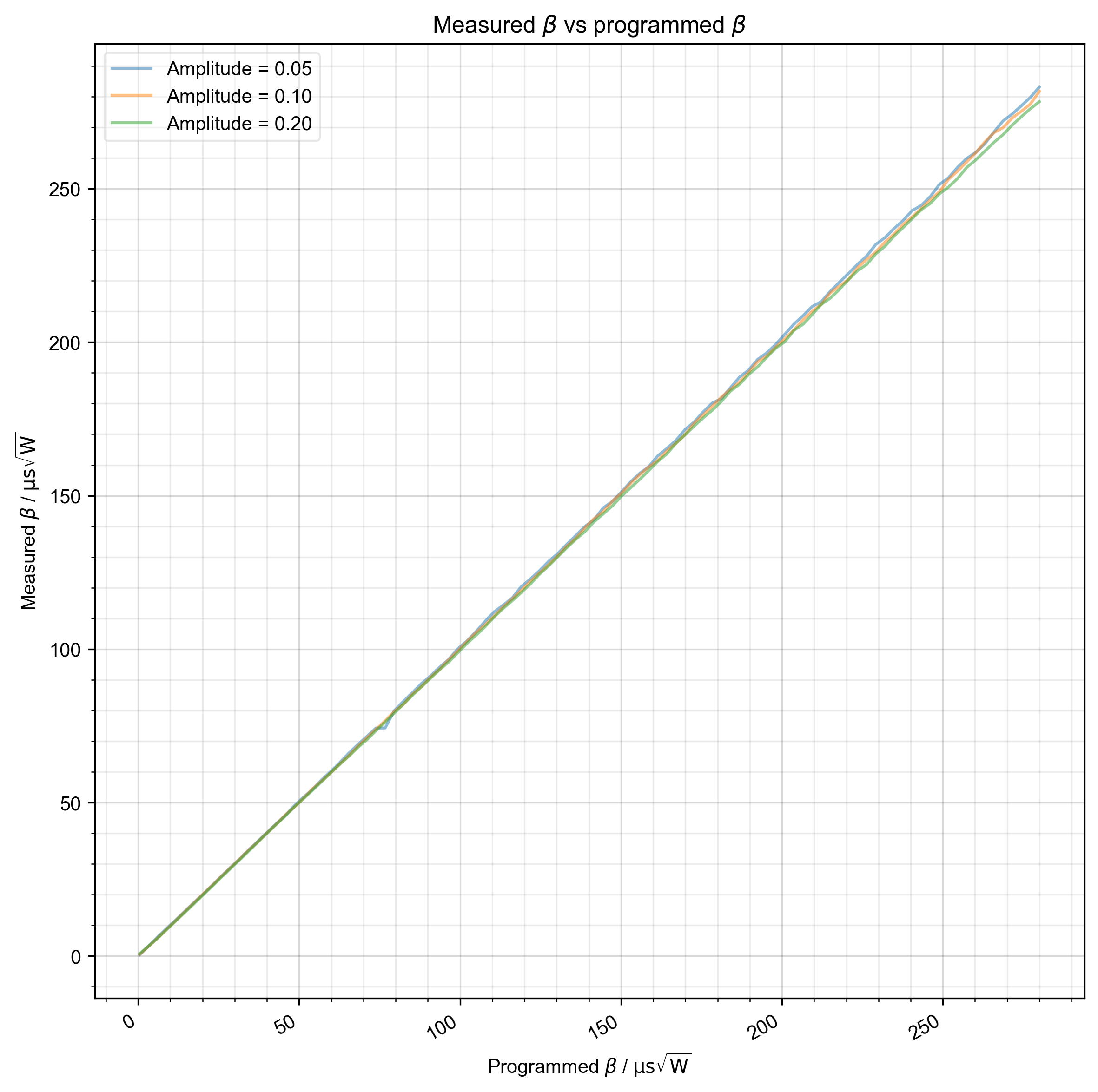
Verify the pulse calibration

Once we have the pulse-length calibration in place, we want to simply verify that we get the β values that we program, where \(\beta = \frac{1}{\sqrt{2} \int \sqrt{P(t)_{amp}} dt\)

This data should be acquired using example/run_pulse_calibration.py in FLInst.

Compare to example/calibrate_tsqrtP.py, which generates the calibration.

• 
• 
• 
• 
• 
• 
• 
• 
• 
• 
• 
• 
• 
• 
• 
• 
• 

----------  logging output to /home/jmfranck/pyspecdata.0.log  ----------
You didn't set units for beta before saving the data!!!
--> simple_functions.py(126):root find_apparent_anal_freq 2024-10-26 15:48:51,629
INFO: Aliasing occurred, but we can still find that frequency!
You didn't set units for beta before saving the data!!!
You didn't set units for beta before saving the data!!!
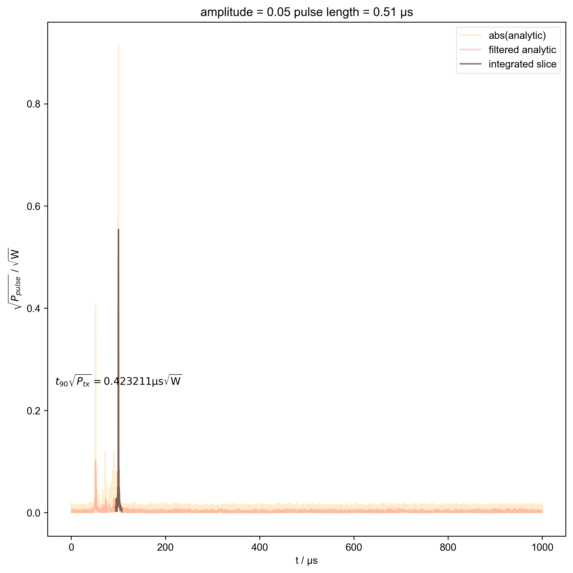
1: amplitude = 0.05 pulse length = 0.51 μs |||μs
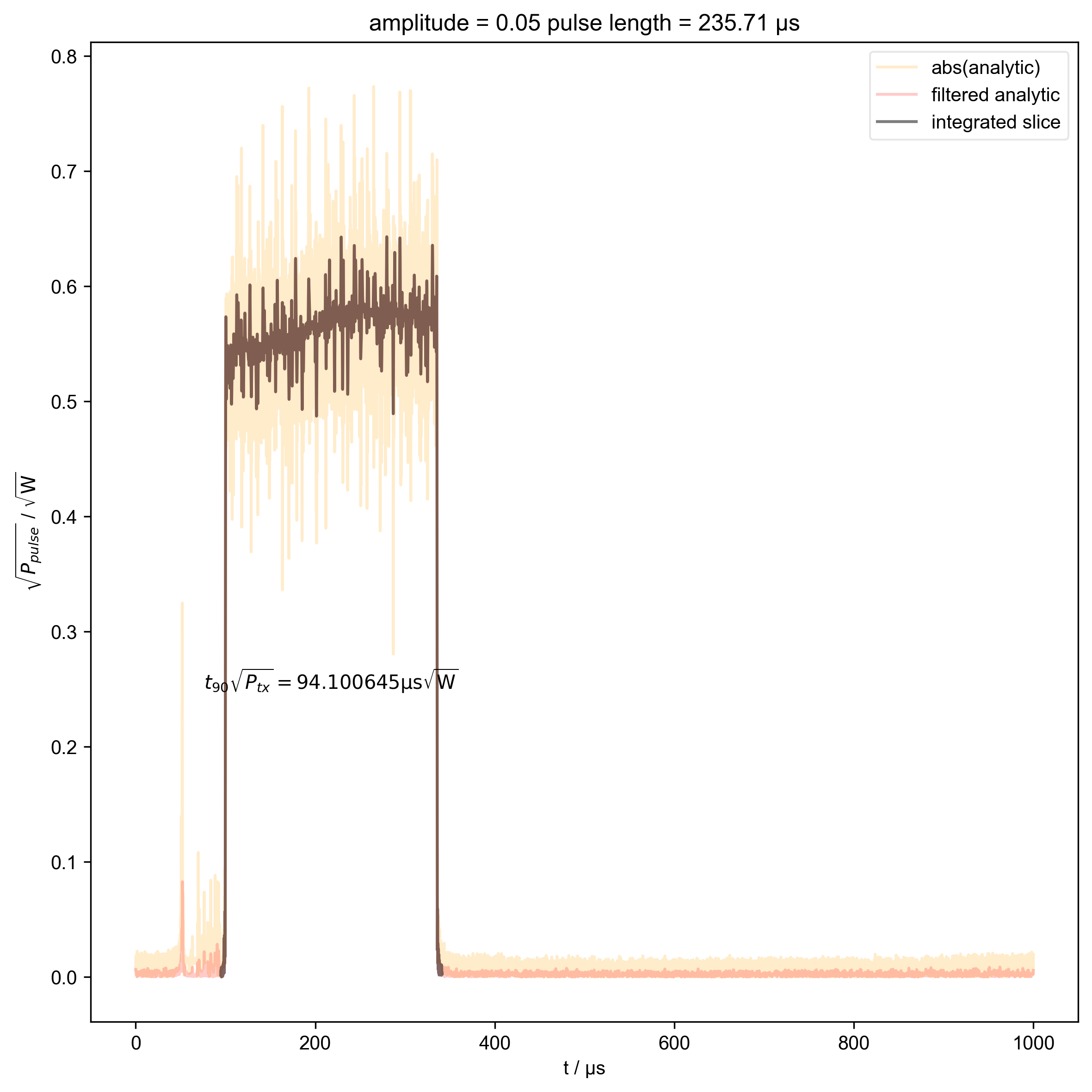
2: amplitude = 0.05 pulse length = 235.71 μs |||μs
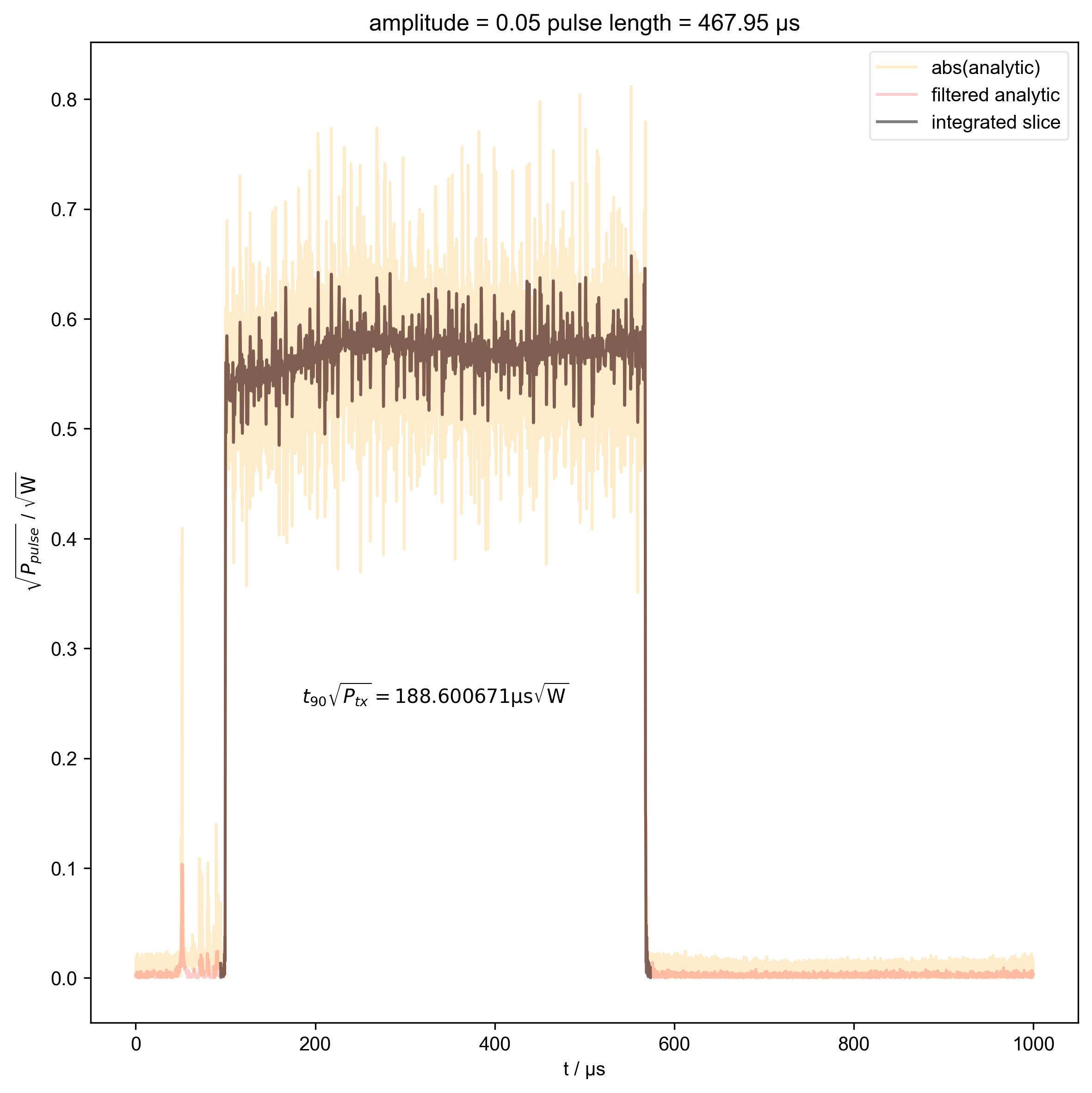
3: amplitude = 0.05 pulse length = 467.95 μs |||μs
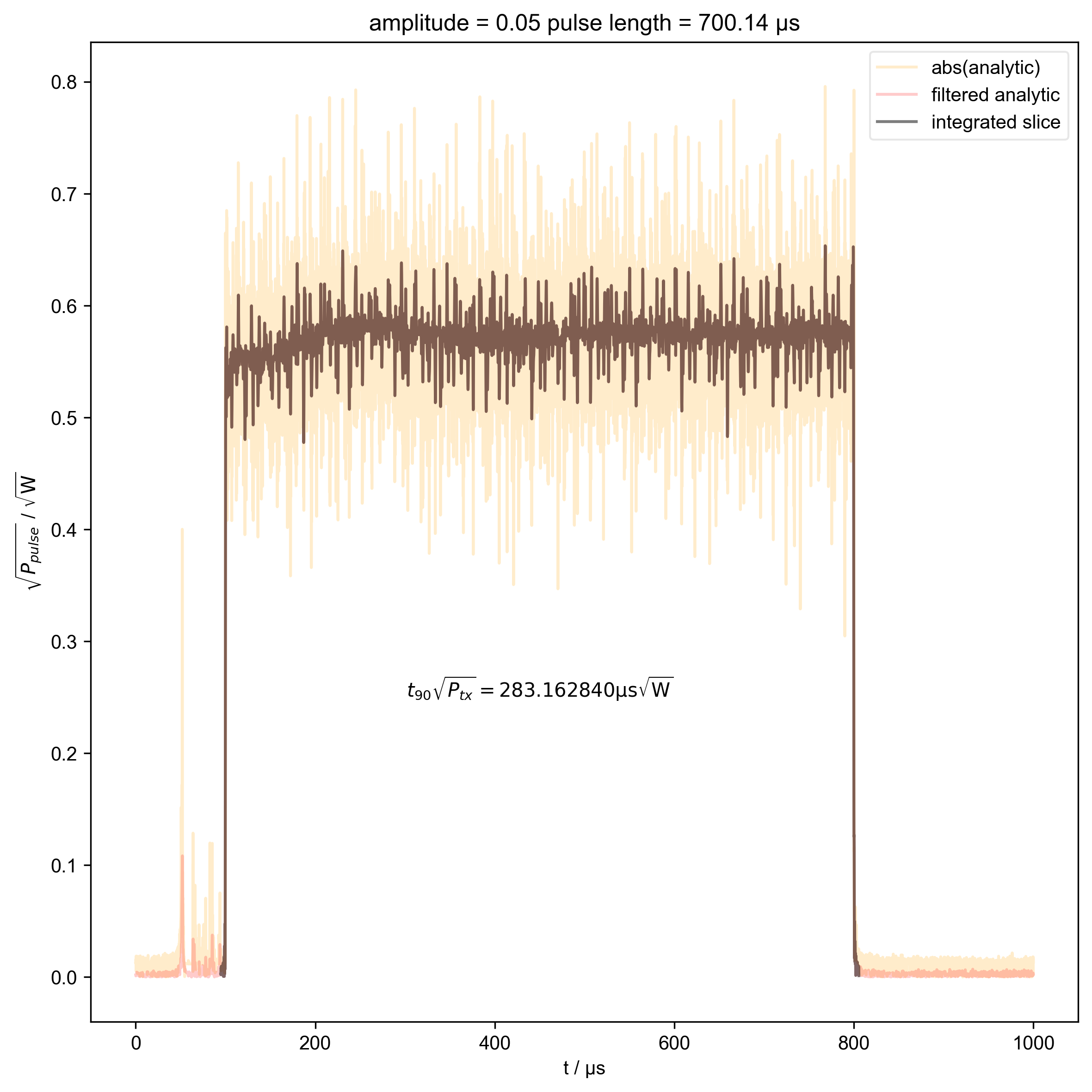
4: amplitude = 0.05 pulse length = 700.14 μs |||μs
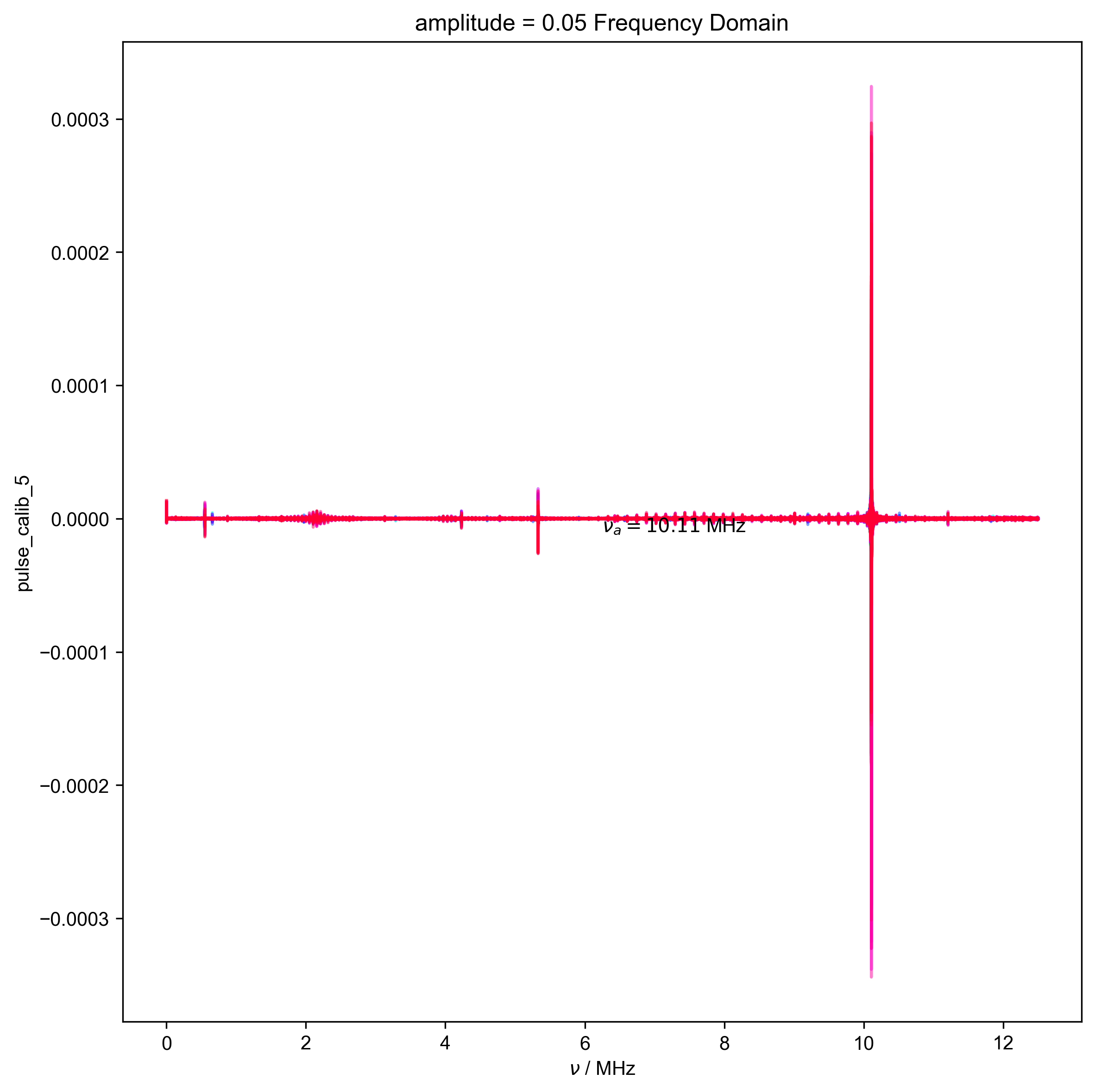
5: amplitude = 0.05 Frequency Domain |||('MHz', None)
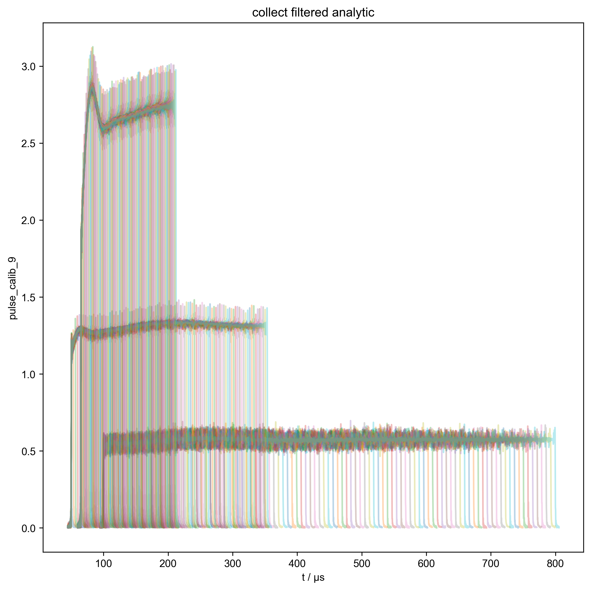
6: collect filtered analytic |||μs
7: Measured $\beta$ vs programmed $\beta$ |||μs√W
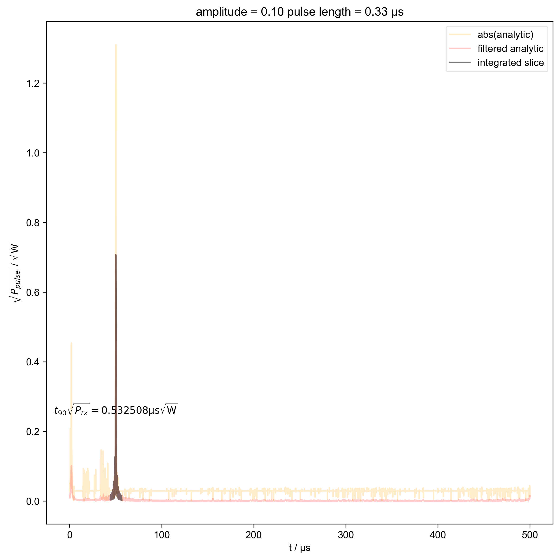
8: amplitude = 0.10 pulse length = 0.33 μs |||μs
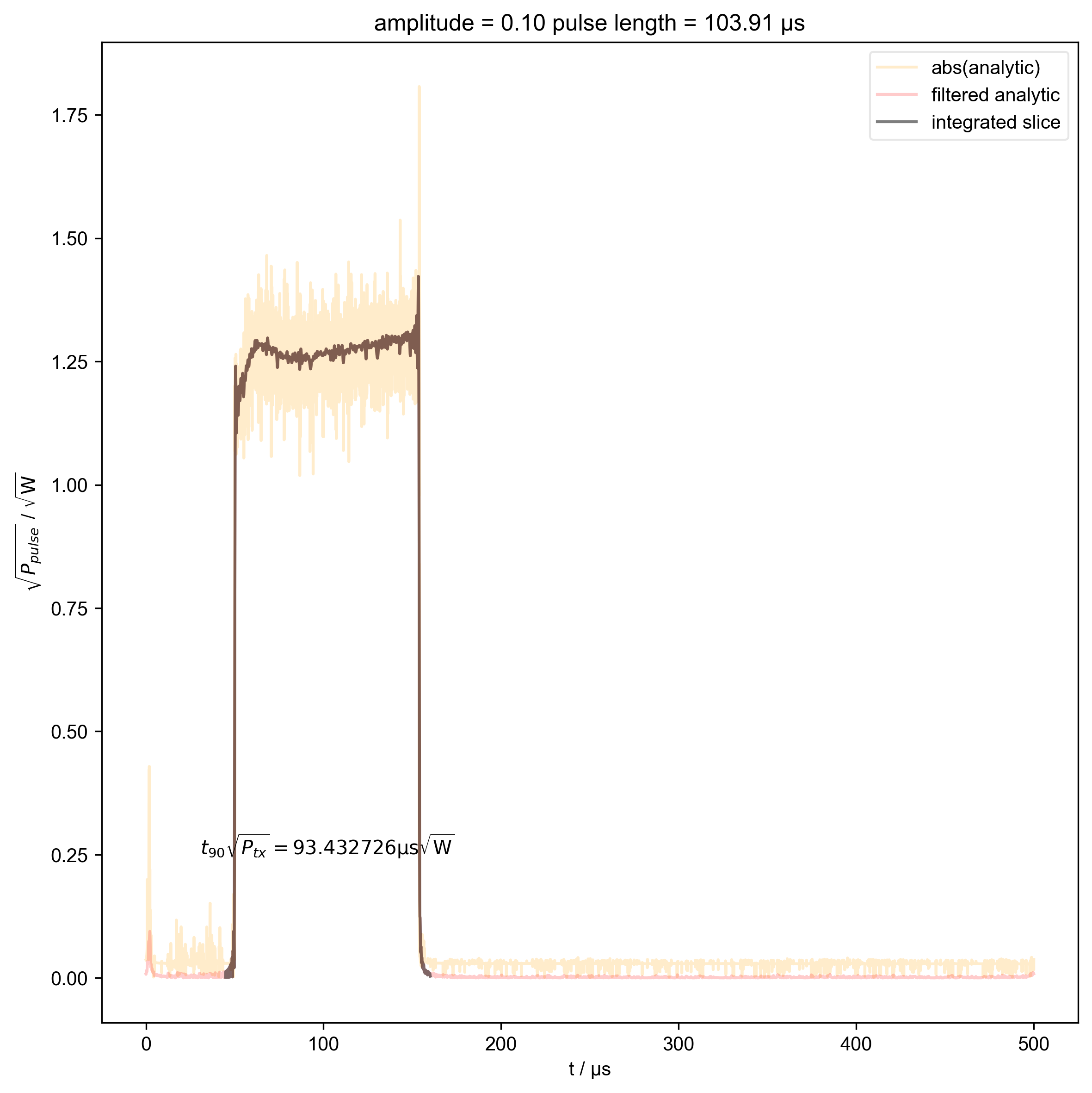
9: amplitude = 0.10 pulse length = 103.91 μs |||μs
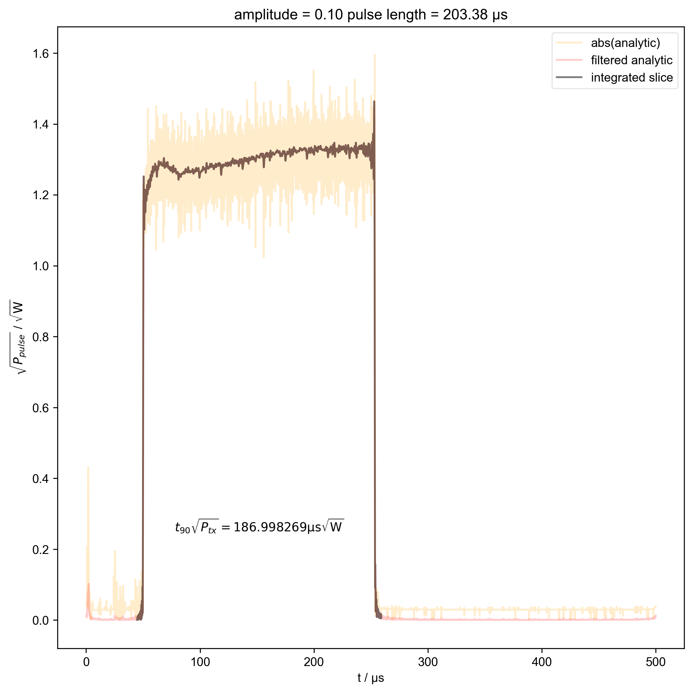
10: amplitude = 0.10 pulse length = 203.38 μs |||μs
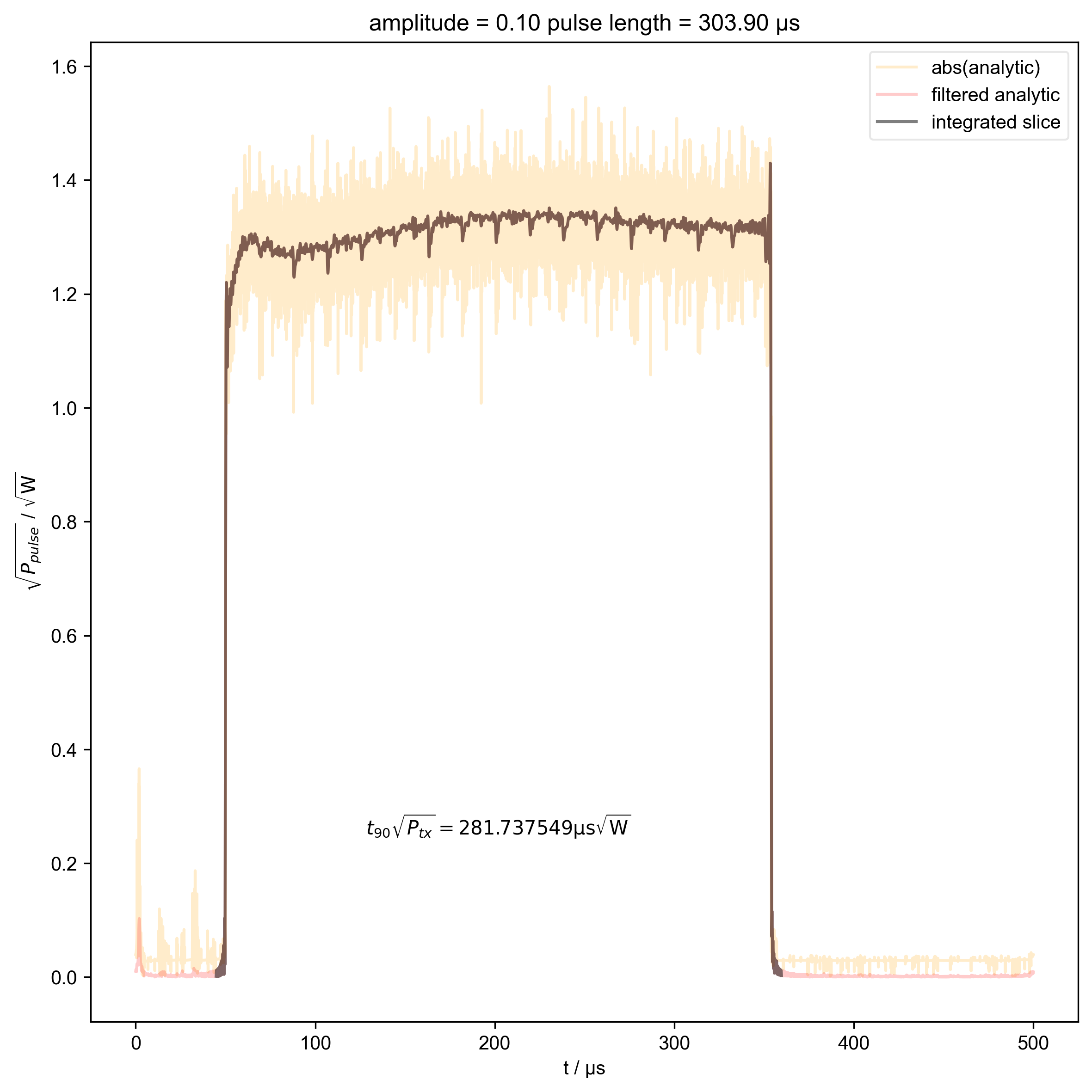
11: amplitude = 0.10 pulse length = 303.90 μs |||μs
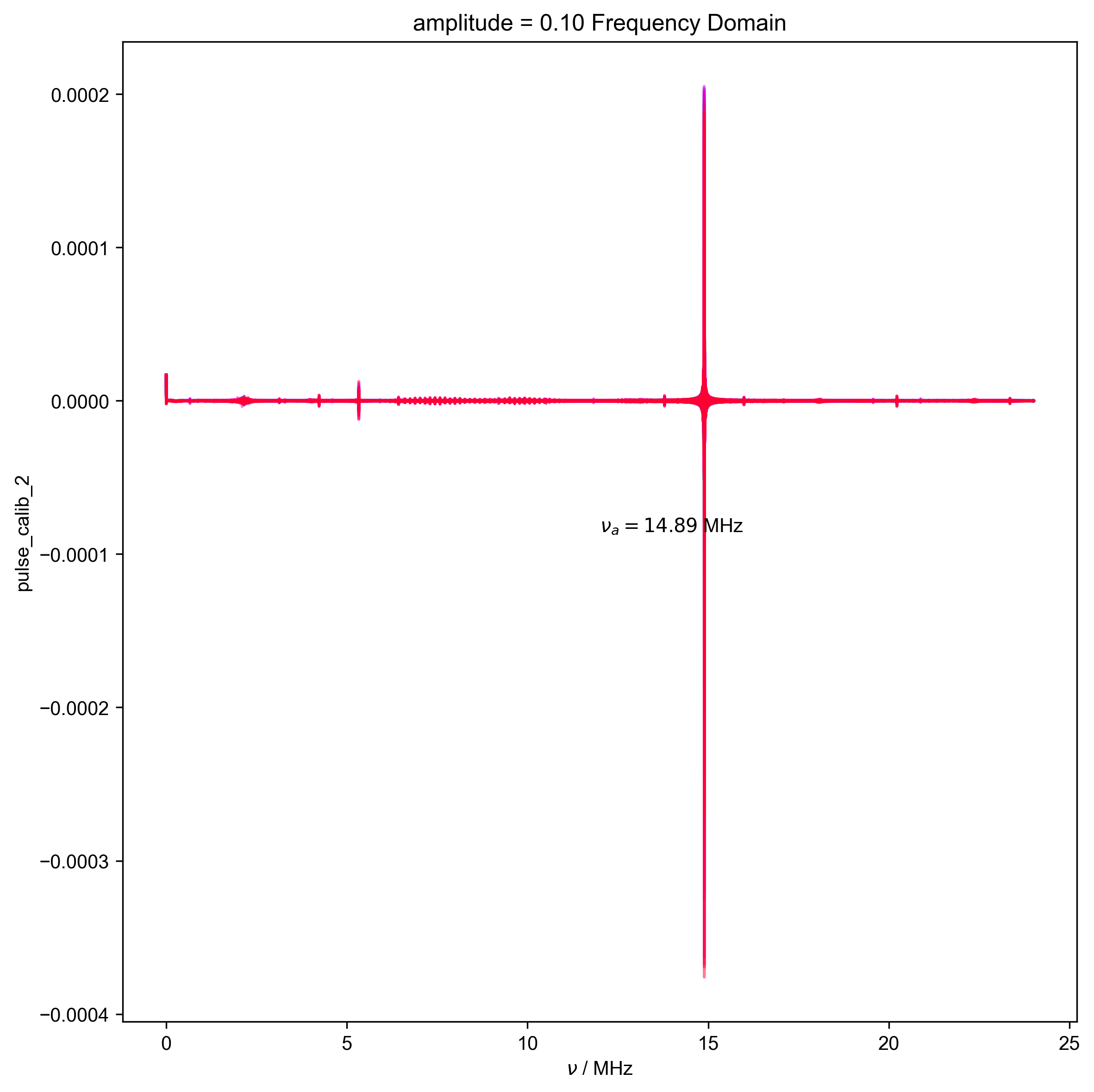
12: amplitude = 0.10 Frequency Domain |||('MHz', None)
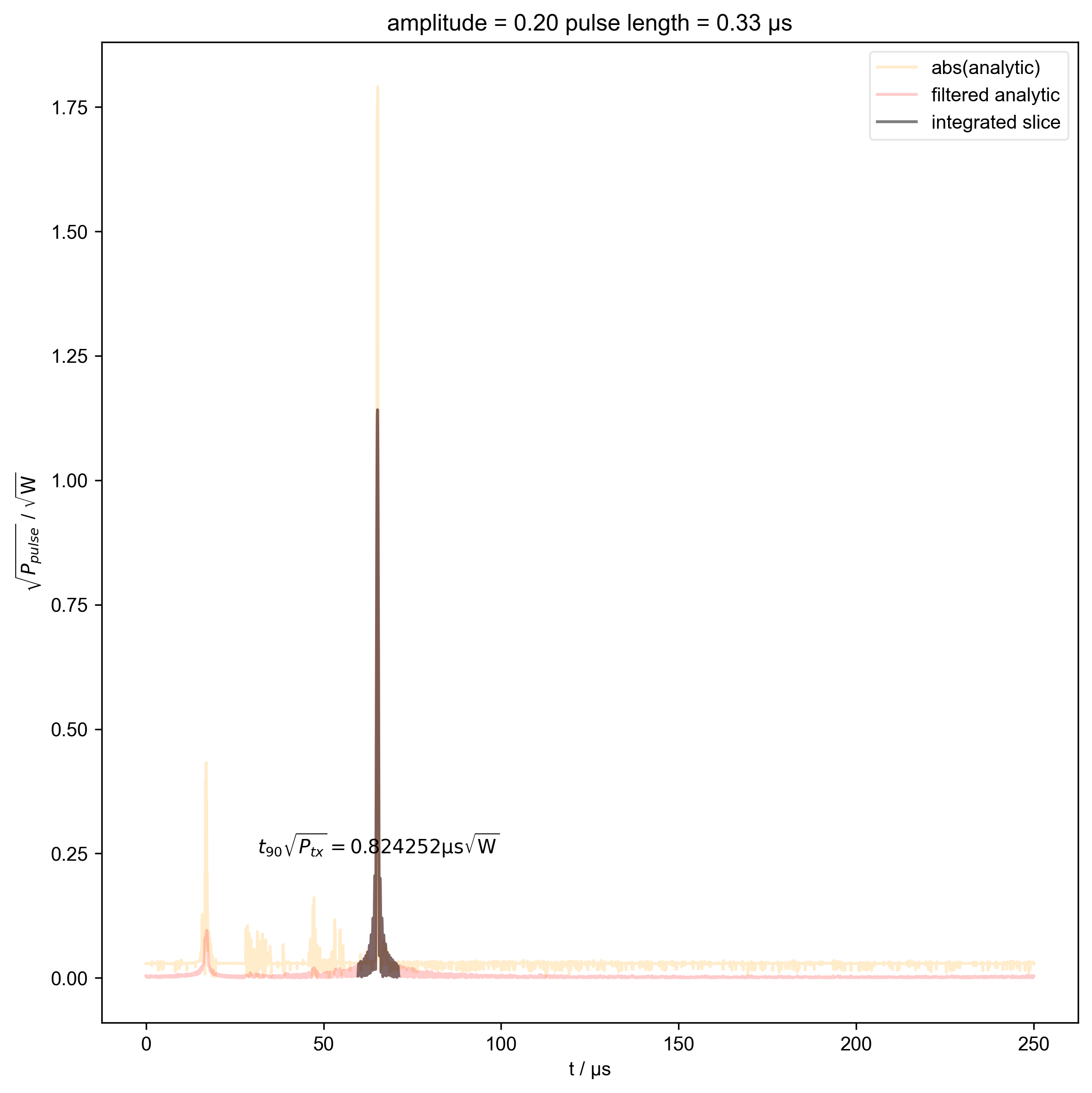
13: amplitude = 0.20 pulse length = 0.33 μs |||μs
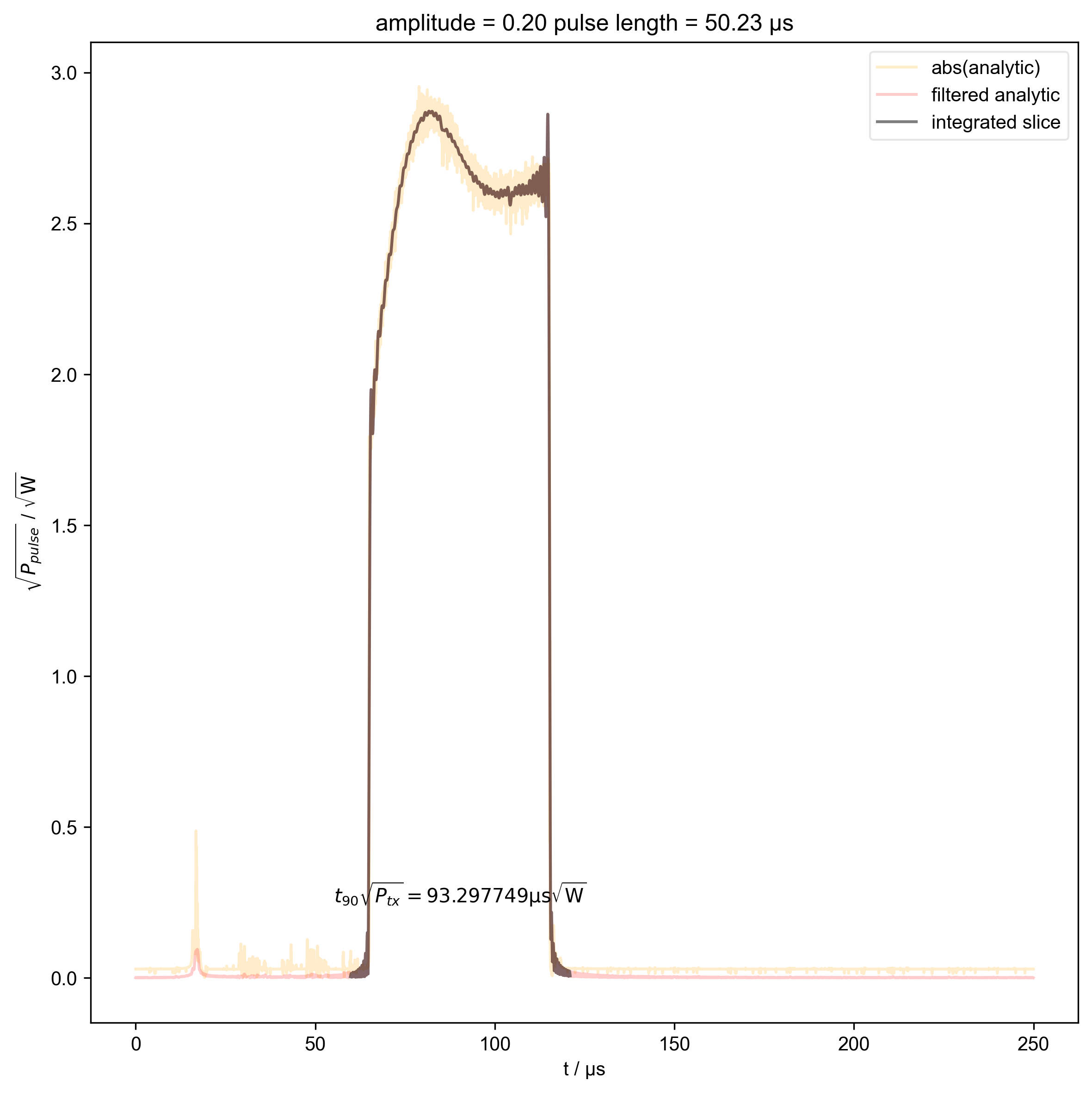
14: amplitude = 0.20 pulse length = 50.23 μs |||μs
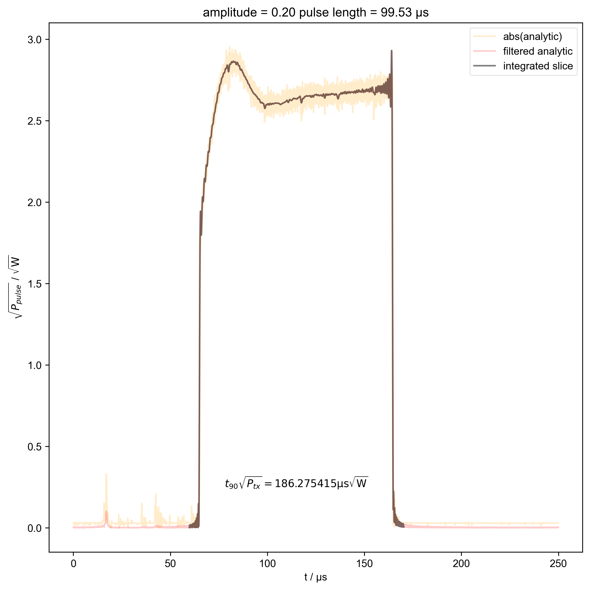
15: amplitude = 0.20 pulse length = 99.53 μs |||μs
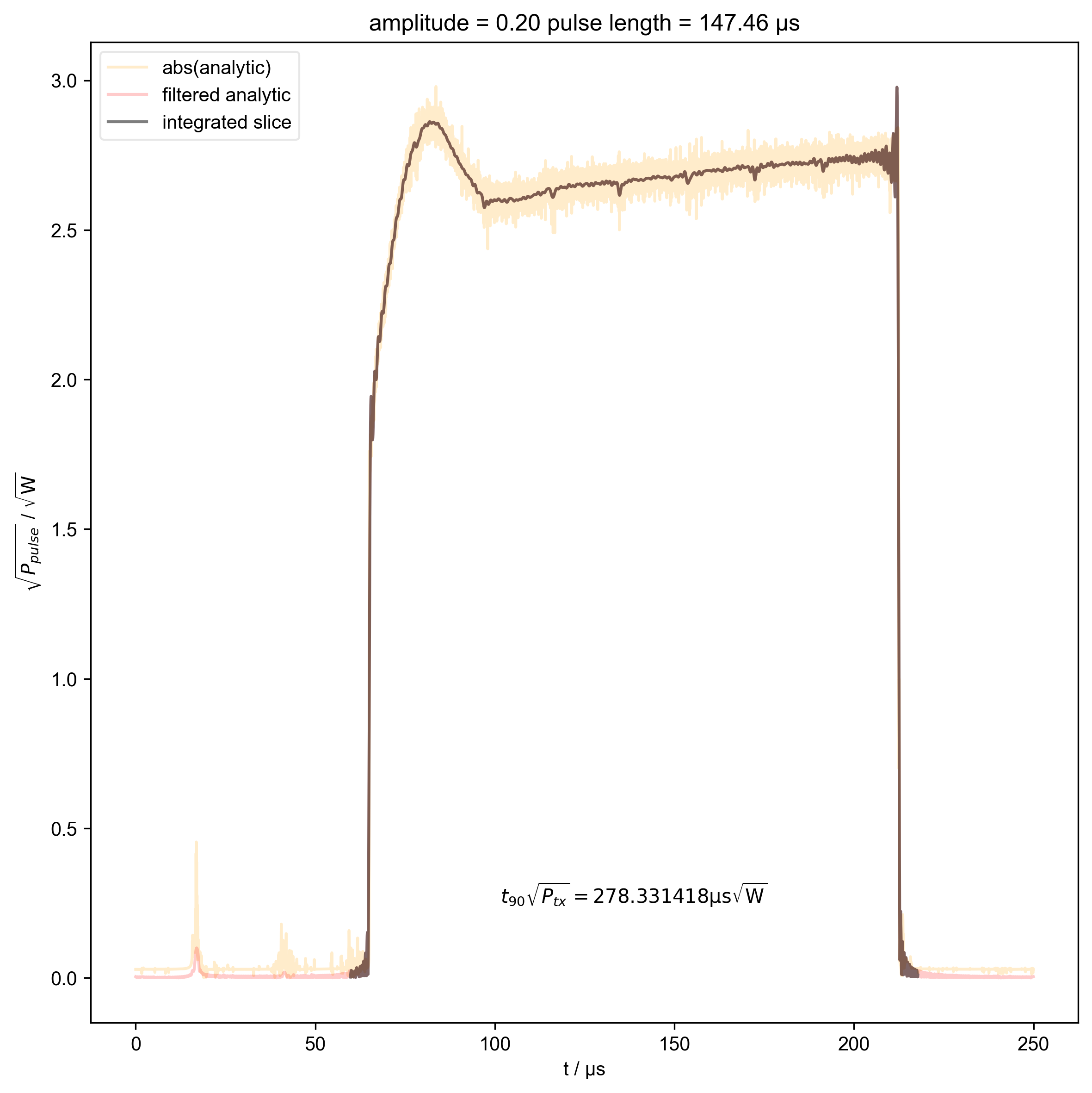
16: amplitude = 0.20 pulse length = 147.46 μs |||μs
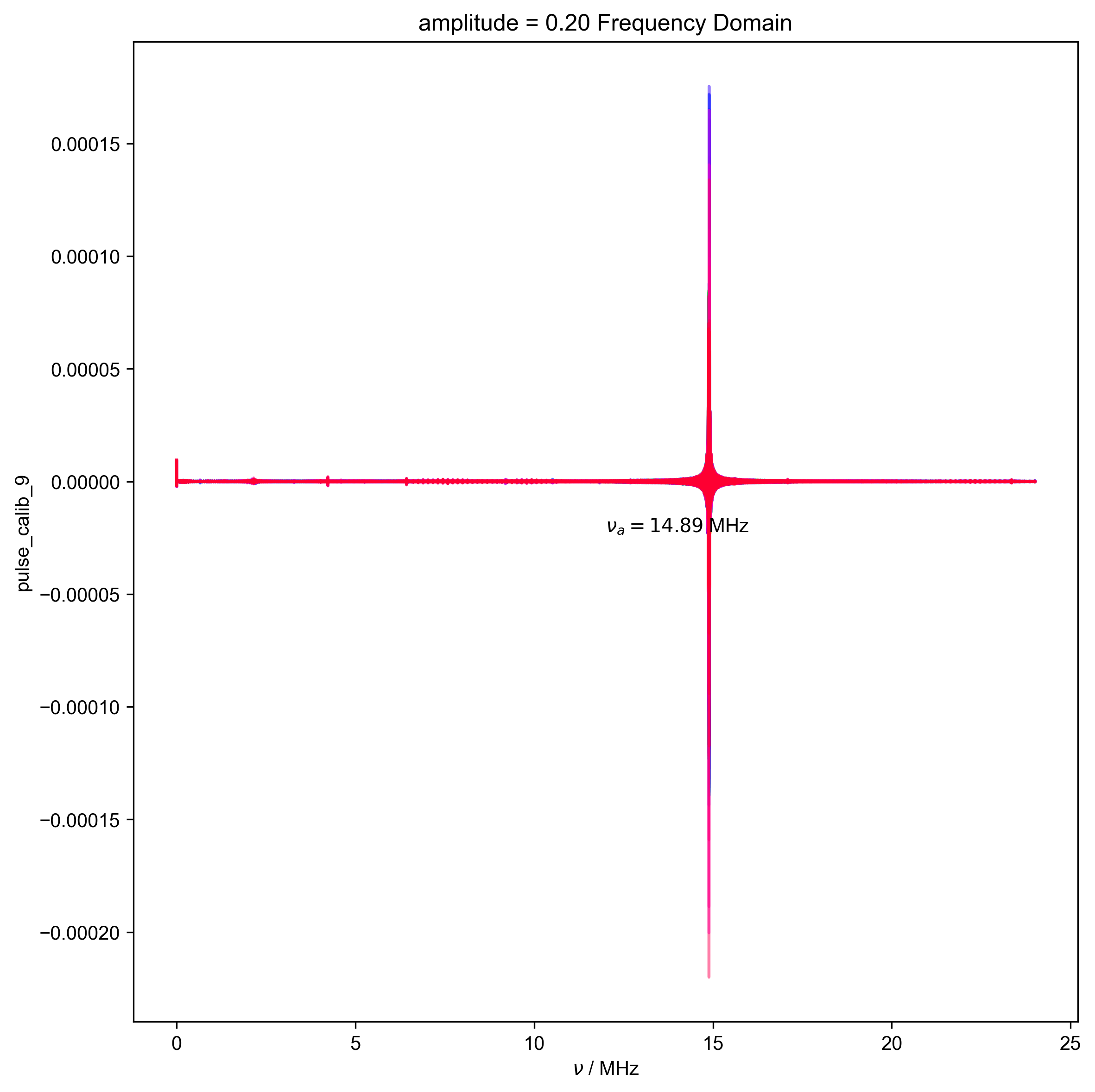
17: amplitude = 0.20 Frequency Domain |||('MHz', None)

import pyspecdata as psd
from pyspecProcScripts import find_apparent_anal_freq
import matplotlib.pyplot as plt
import numpy as np
from itertools import cycle

psd.init_logging()

colorcyc_list = plt.rcParams["axes.prop_cycle"].by_key()["color"]
color_cycle = cycle(
    colorcyc_list
)  # this can be done more than once to spin up multiple lists

V_atten_ratio = 102.2  # attenutation ratio
skip_plots = 33  # diagnostic -- set this to None, and there will be no
#                  plots
HH_width = 2e6


with psd.figlist_var() as fl:
    for filename, nodename in [
        (
            "240819_test_amp0p05_calib_pulse_calib.h5",
            "pulse_calib_5",
        ),
        (
            "240819_amp0p1_calib_pulse_calib.h5",
            "pulse_calib_2",
        ),
        (
            "240819_amp0p2_calib_repeat_pulse_calib.h5",
            "pulse_calib_9",
        ),
    ]:
        d = psd.find_file(
            filename, expno=nodename, exp_type="ODNP_NMR_comp/test_equipment"
        )
        assert (
            d.get_prop("postproc_type") == "GDS_capture_v1"
        ), "The wrong postproc_type was set so you most likely used the wrong script for acquisition"
        amplitude = d.get_prop("acq_params")["amplitude"]
        fl.basename = f"amplitude = {amplitude:.2f}"
        d *= V_atten_ratio  # V at output of amplifier
        d /= np.sqrt(50)  # V/sqrt(R) = sqrt(P_amp)

        # {{{ functions that streamline plotting the desired pulse length
        #     datasets
        def switch_to_plot(d, j):
            thislen = d.get_prop("programmed_t_pulse")[j] / 1e-6
            fl.next(f"pulse length = {thislen:.2f} μs")

        def indiv_plots(d, thislabel, thiscolor):
            if skip_plots is None:
                return
            for j in range(len(d["beta"])):
                if j % skip_plots == 0:
                    switch_to_plot(d, j)
                    fl.plot(
                        d["beta", j],
                        alpha=0.2,
                        color=thiscolor,
                        label=thislabel,
                    )
                    plt.ylabel(r"$\sqrt{P}$ / $\sqrt{\mathrm{W}}$")

        # }}}
        # {{{ data is already analytic, and downsampled to below 24 MHz
        indiv_plots(abs(d), "abs(analytic)", "orange")
        d, nu_a, _ = find_apparent_anal_freq(d)  # find frequency of signal
        d.ft("t")
        # {{{ Diagnostic to ensure the frequency properly identified
        fl.next("Frequency Domain")
        fl.plot(d)
        plt.text(
            x=0.5,
            y=0.5,
            s=rf"$\nu_a={nu_a/1e6:0.2f}$ MHz",
            transform=plt.gca().transAxes,
        )
        assert (0 > nu_a * 0.5 * HH_width) or (
            0 < nu_a - 0.5 * HH_width
        ), "unfortunately the region I want to filter includes DC -- this is probably not good, and you should pick a different timescale for your scope so this doesn't happen"
        # }}}
        # {{{ apply HH frequency filter
        d["t" : (None, nu_a - 0.5 * HH_width)] *= 0
        d["t" : (nu_a + 0.5 * HH_width, None)] *= 0
        # }}}
        d.ift("t")
        indiv_plots(abs(d), "filtered analytic", "red")
        # }}}
        # {{{ set up shape of data to drop the calculated beta values in
        verify_beta = d.shape.pop("t").alloc(dtype=np.float64)
        verify_beta.copy_axes(d)
        verify_beta.set_units(r"s√W").set_units("beta", r"s√W")
        # }}}
        thiscolor = next(color_cycle)
        for j in range(len(d["beta"])):
            s = d["beta", j]
            int_range = abs(s).contiguous(lambda x: x > 0.03 * s.max())[0]
            # slightly expand int range to include rising edges
            int_range[0] -= 5e-6
            int_range[-1] += 5e-6
            # {{{ plot the integration range of all pulses prior to integrating.
            #     Serves as diagnostic to ensure the beta is consistently increasing.
            fl.push_marker()
            fl.basename = None
            fl.next("collect filtered analytic")
            fl.plot(abs(s["t":int_range]), alpha=0.3)
            fl.pop_marker()
            # }}}
            verify_beta["beta", j] = abs(s["t":int_range]).integrate(
                "t"
            ).data.item() / np.sqrt(
                2
            )  # tp * sqrt(P_rms)
            # {{{ Can't use indiv_plots because we've already indexed the beta
            # out and we also want to plot the calculated beta on top
            if skip_plots is not None and j % skip_plots == 0:
                switch_to_plot(d, j)
                fl.plot(
                    abs(s["t":int_range]),
                    color="black",
                    label="integrated slice",
                )
                plt.ylabel(r"$\sqrt{P_{pulse}}$ / $\sqrt{\mathrm{W}}$")
                plt.text(
                    np.mean(int_range) / 1e-6,
                    0.25,
                    r"$t_{90} \sqrt{P_{tx}} = %f \mathrm{μs} \sqrt{\mathrm{W}}$"
                    % (verify_beta["beta", j].item() / 1e-6),
                    ha="center",
                )
            # }}}
        # {{{ show what we observe -- how does β vary with the desired β
        fl.basename = None  # we want to plot all amplitudes together now
        fl.next(r"Measured $\beta$ vs programmed $\beta$")
        fl.plot(
            (verify_beta / 1e-6).set_units("μs√W"),
            color=thiscolor,
            label="Amplitude = %0.2f" % amplitude,
        )
        plt.xlabel(r"Programmed $\beta$ / $\mathrm{μs}\sqrt{\mathrm{W}}$")
        plt.ylabel(r"Measured $\beta$ / $\mathrm{μs}\sqrt{\mathrm{W}}$")
        psd.gridandtick(plt.gca())
        # }}}