Calculating β from individual pulse capture

Assuming a single pulse was acquired via simple_onepulse_capture.py in the FLInst repo using the GDS oscilloscope, this script plots the absolute analytic along with the frequency filtered absolute of the analytic before integrating to calculate :math:`beta = frac{1}{sqrt{2}}int{V(t)dt}’.

• 
• 
• 
• 
• 
• 

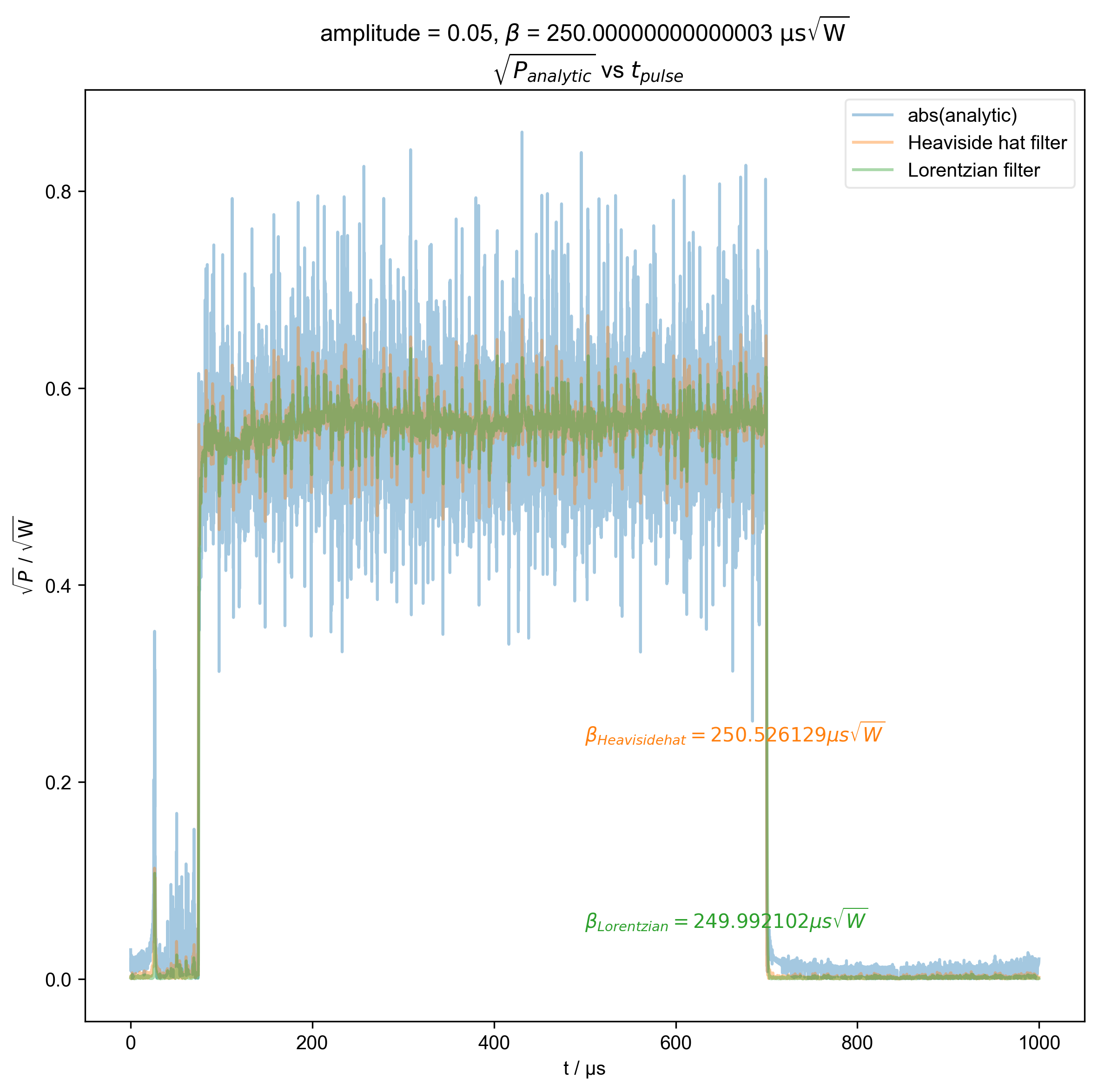
1: amplitude = 0.05, ${\beta}$ = 250.00000000000003 ${\mathrm{\mu s \sqrt{W}}}$
 $\sqrt{P_{analytic}}$ vs $t_{pulse}$ |||μs
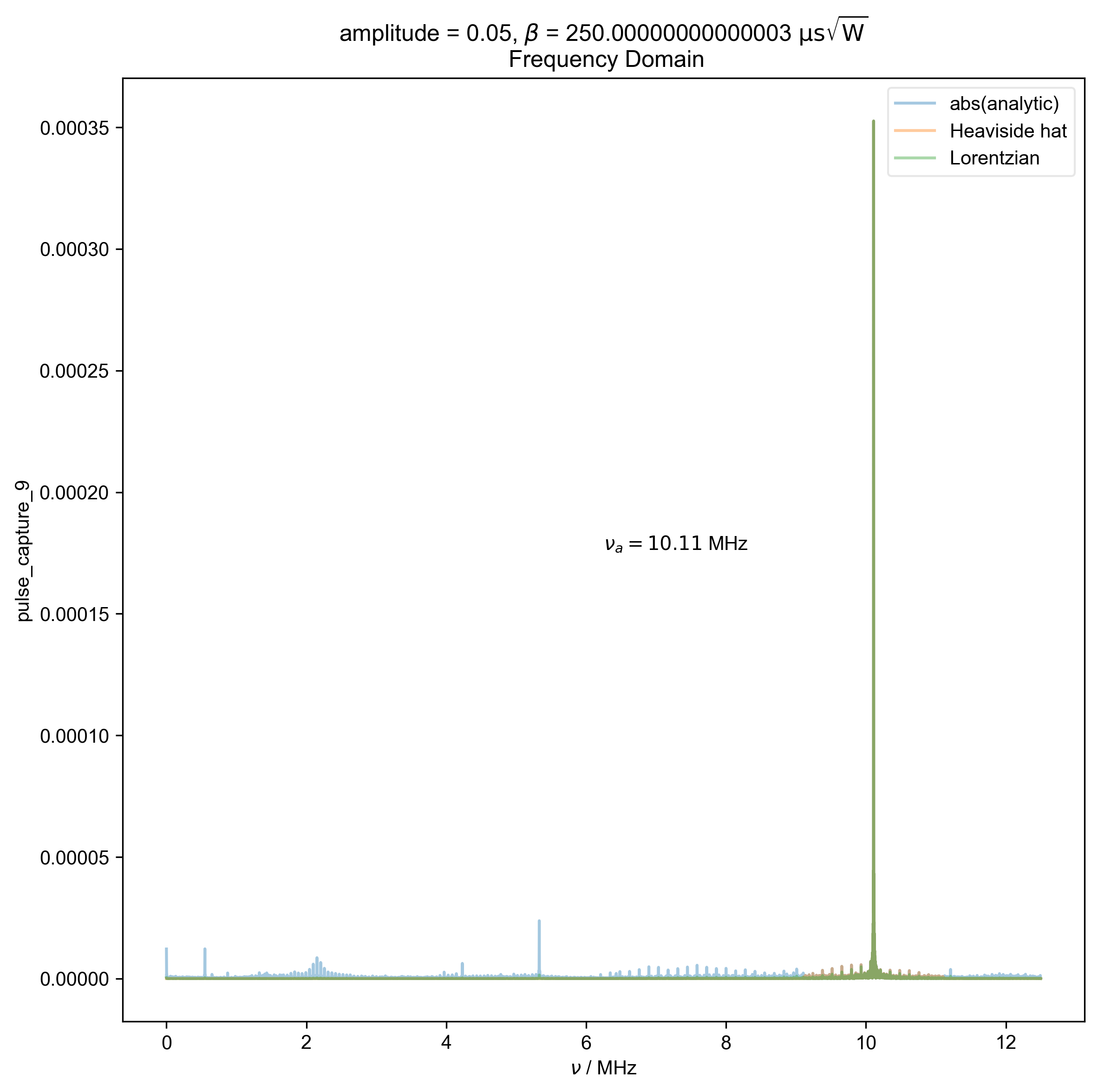
2: amplitude = 0.05, ${\beta}$ = 250.00000000000003 ${\mathrm{\mu s \sqrt{W}}}$
 Frequency Domain |||MHz
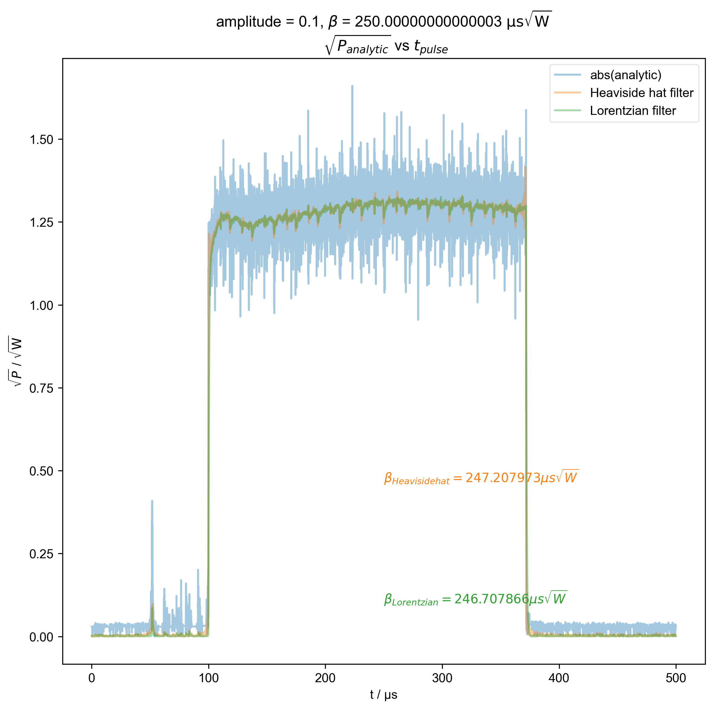
3: amplitude = 0.1, ${\beta}$ = 250.00000000000003 ${\mathrm{\mu s \sqrt{W}}}$
 $\sqrt{P_{analytic}}$ vs $t_{pulse}$ |||μs
4: amplitude = 0.1, ${\beta}$ = 250.00000000000003 ${\mathrm{\mu s \sqrt{W}}}$
 Frequency Domain |||MHz
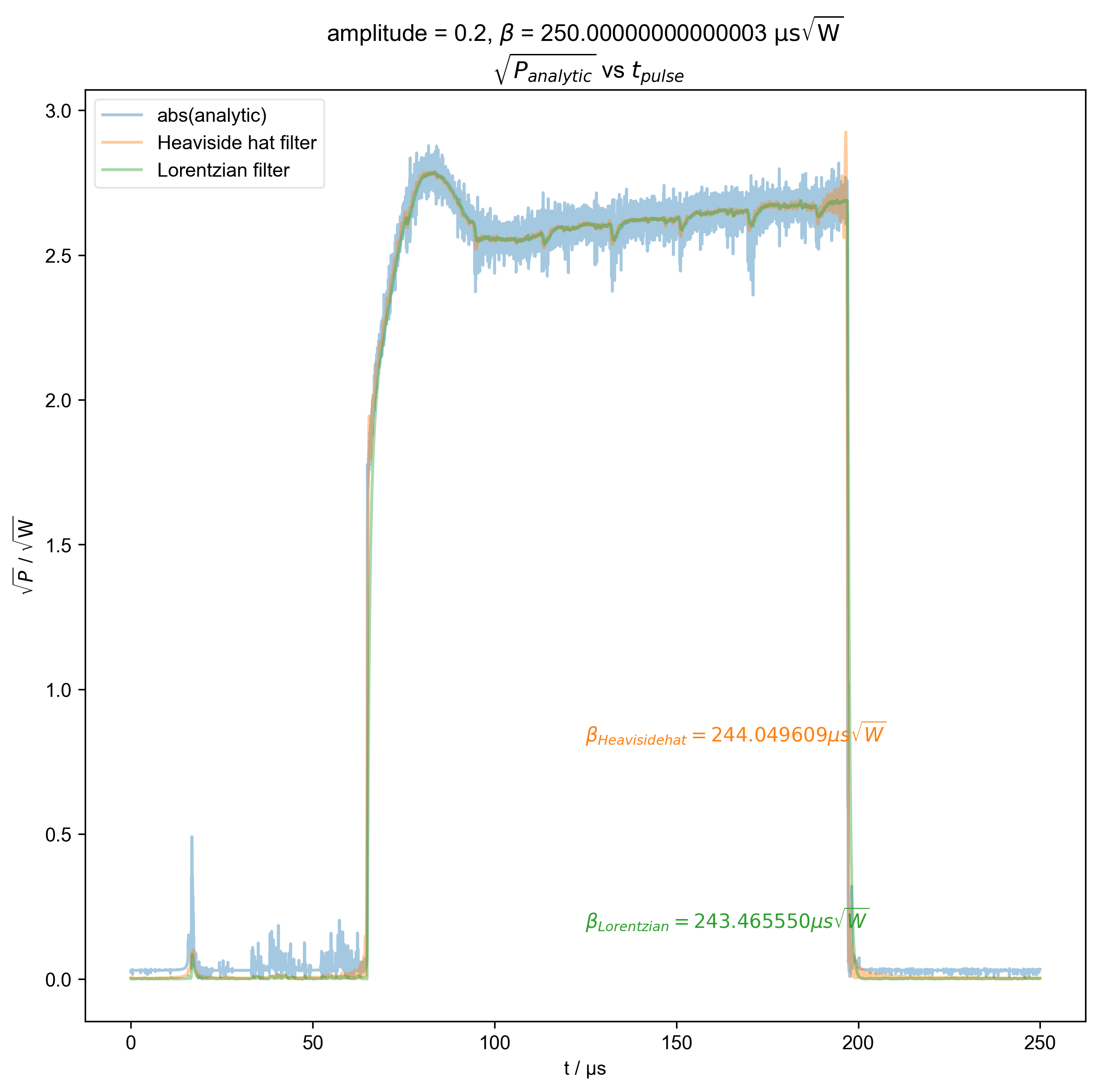
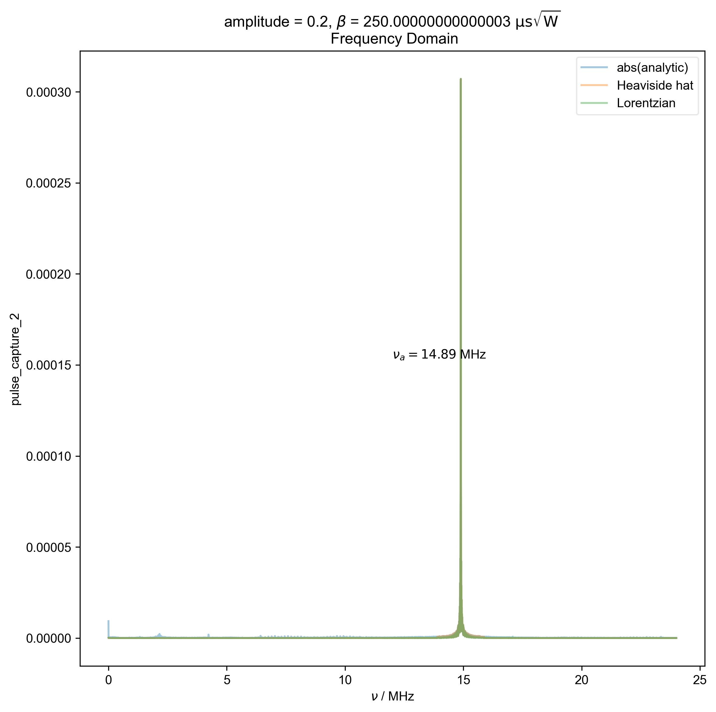
5: amplitude = 0.2, ${\beta}$ = 250.00000000000003 ${\mathrm{\mu s \sqrt{W}}}$
 $\sqrt{P_{analytic}}$ vs $t_{pulse}$ |||μs
6: amplitude = 0.2, ${\beta}$ = 250.00000000000003 ${\mathrm{\mu s \sqrt{W}}}$
 Frequency Domain |||MHz

import pyspecdata as psd
import matplotlib.pyplot as plt
import numpy as np
from itertools import cycle
from pyspecProcScripts import find_apparent_anal_freq

colorcyc_list = plt.rcParams["axes.prop_cycle"].by_key()["color"][:3]
color_cycle = cycle(colorcyc_list)

V_atten_ratio = 102.2  # attenutation ratio
HH_width = 2e6
Delta_nu = (
    15.19e6 - 14.61e6
)  # width of reflection at -3dB - specific to large probe

with psd.figlist_var() as fl:
    for filename, nodename in [
        (
            "240819_amp0p05_beta_max_pulse_capture.h5",
            "pulse_capture_9",
        ),
        (
            "240819_amp0p1_beta_max_pulse_capture.h5",
            "pulse_capture_6",
        ),
        (
            "240819_amp0p2_beta_max_pulse_capture.h5",
            "pulse_capture_2",
        ),
    ]:
        s = psd.find_file(
            filename, expno=nodename, exp_type="ODNP_NMR_comp/test_equipment"
        )
        # {{{ define basename
        amplitude = s.get_prop("acq_params")["amplitude"]
        fl.basename = f"amplitude = {amplitude}, ${{\\beta}}$ = {s.get_prop('acq_params')['beta_90_s_sqrtW'] / 1e-6} ${{\\mathrm{{\\mu s \\sqrt{{W}}}}}}$ \n"
        # }}}
        if not s.get_units("t") == "s":
            print(
                "units weren't set for the t axis or else I can't read them from the hdf5 file!"
            )
            s.set_units("t", "s")
        s *= V_atten_ratio  # attenutation ratio
        s /= np.sqrt(50)  # V/sqrt(R) = sqrt(P)
        # {{{ plot absolute analytic
        fl.next(r"$\sqrt{P_{analytic}}$ vs $t_{pulse}$")
        thiscolor = next(color_cycle)
        fl.plot(abs(s), color=thiscolor, alpha=0.4, label="abs(analytic)")
        # }}}
        # {{{ apply frequency filter
        s, nu_a, _ = find_apparent_anal_freq(s)
        assert (0 > nu_a * 0.5 * HH_width) or (
            0 < nu_a - 0.5 * HH_width
        ), "unfortunately the region I want to filter includes DC -- this is probably not good, and means you should pick a different timescale for your scope so this doesn't happen"
        s.ft("t")
        # {{{ Display frequency domain
        fl.next("Frequency Domain")
        fl.plot(abs(s), color=thiscolor, alpha=0.4, label="abs(analytic)")
        plt.text(
            x=0.5,
            y=0.5,
            s=rf"$\nu_a={nu_a/1e6:0.2f}$ MHz",
            transform=plt.gca().transAxes,
        )
        # }}}
        # {{{ lorentzian filter
        Lorentzian_filtered = s / (
            1 + 1j * 2 * (s.fromaxis("t") - nu_a) * (1 / Delta_nu)
        )
        # }}}
        # {{{ heaviside hat functions
        s["t" : (None, nu_a - 0.5 * HH_width)] *= 0
        s["t" : (nu_a + 0.5 * HH_width, None)] *= 0
        # }}}
        # }}}
        # {{{ plot application of all filters
        for filtered_data, label, ax_place in [
            (s, "Heaviside hat", 0.3),
            (Lorentzian_filtered, "Lorentzian", 0.1),
        ]:
            thiscolor = next(color_cycle)
            filtered_data.ift("t")
            fl.next(r"$\sqrt{P_{analytic}}$ vs $t_{pulse}$")
            fl.plot(
                abs(filtered_data),
                color=thiscolor,
                alpha=0.4,
                label=label + " filter",
            )
            filtered_data.ft("t")
            fl.next("Frequency Domain")
            fl.plot(
                abs(filtered_data), color=thiscolor, alpha=0.4, label=label
            )
            filtered_data.ift("t")
            beta = abs(filtered_data).integrate("t").data.item() / np.sqrt(2)
            fl.next(r"$\sqrt{P_{analytic}}$ vs $t_{pulse}$")
            plt.text(
                0.5,
                ax_place,
                r"$\beta_{%s} = %f \mu s \sqrt{W}$" % (label, beta / 1e-6),
                color=thiscolor,
                transform=plt.gca().transAxes,
            )
        plt.ylabel(r"$\sqrt{P}$ / $\mathrm{\sqrt{W}}$")
        # }}}