Process nutation data

py proc_nutation.py NODENAME FILENAME EXP_TYPE

Fourier transforms (and any needed data corrections for older data) are performed according to the postproc_type attribute of the data node. This script plots the result as well as examines the phase variation along the indirect dimension. Finally, the data is integrated and fit to a sin**3 function to find the optimal beta_ninety.

Tested with:

py proc_nutation.py nutation_1 240805_amp0p1_27mM_TEMPOL_nutation.h5        ODNP_NMR_comp/nutation

• 
• 
• 
• 
• 

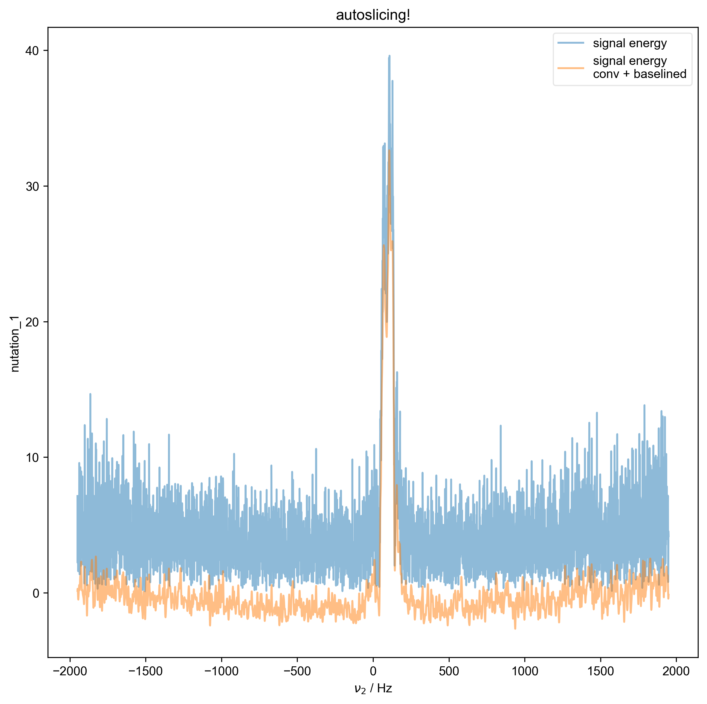
1: autoslicing!
2: Raw Data with averaged scans
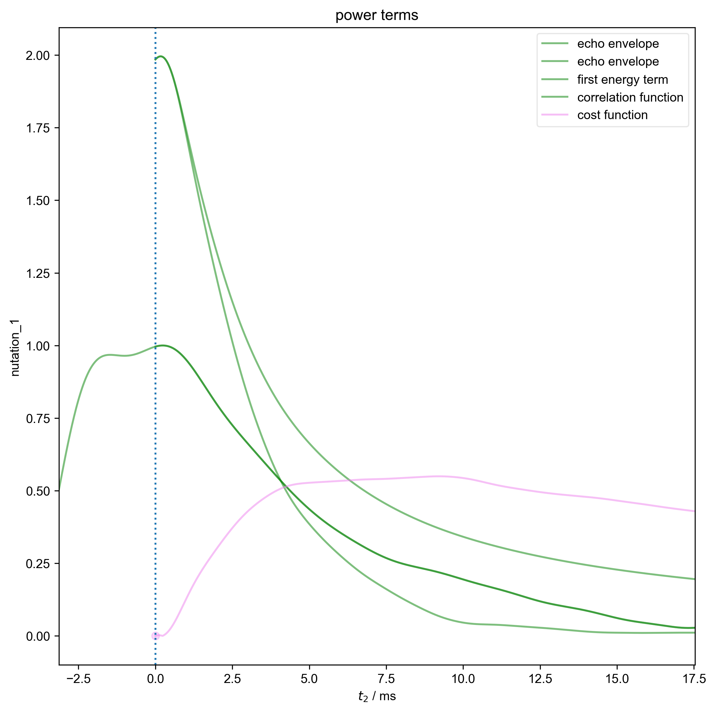
3: power terms |||ms
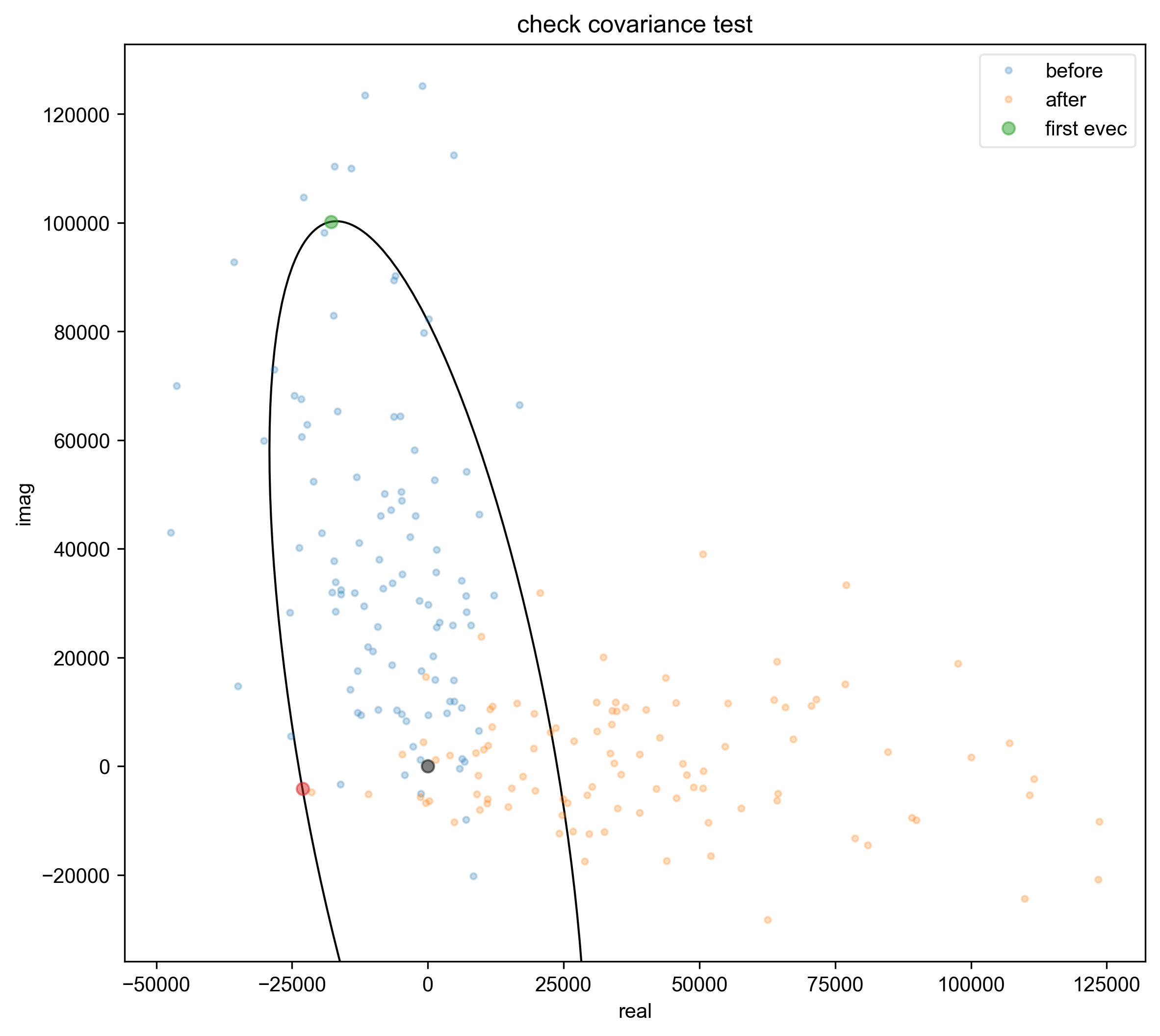
4: check covariance test
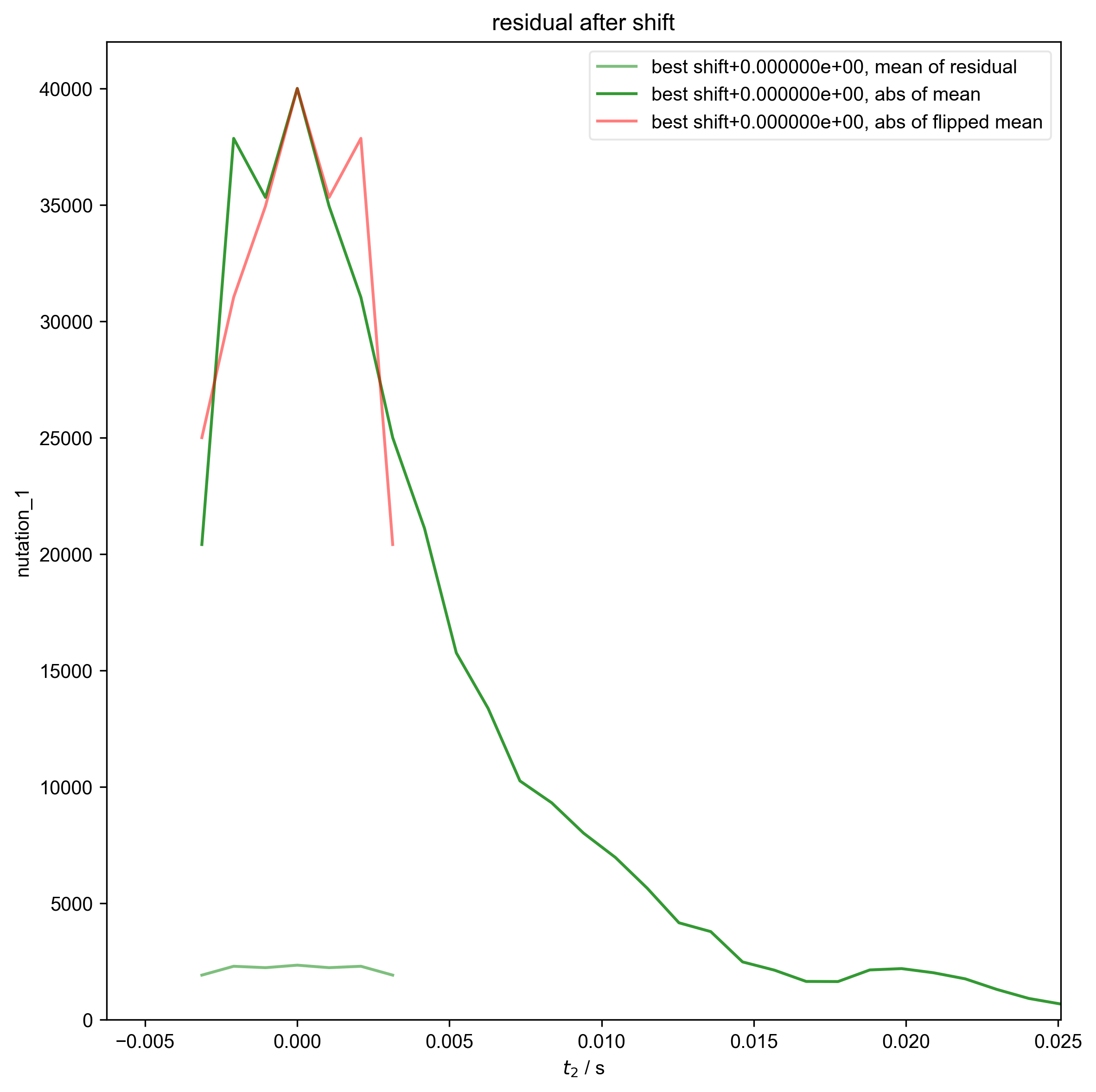
5: residual after shift |||('Hz', 'μs√W')

import pyspecdata as psd
import pyspecProcScripts as prscr
import sympy as sp
import sys, os
from numpy import r_

# even though the following comes from pint, import the instance from
# pyspecdata, because we might want to mess with it.
from pyspecdata import Q_

if (
    "SPHINX_GALLERY_RUNNING" in os.environ
    and os.environ["SPHINX_GALLERY_RUNNING"] == "True"
):
    sys.argv = [
        sys.argv[0],
        "nutation_1",
        "240805_amp0p1_27mM_TEMPOL_nutation.h5",
        "ODNP_NMR_comp/nutation",
    ]

slice_expansion = 5
assert len(sys.argv) == 4
s = psd.find_file(
    sys.argv[2],
    exp_type=sys.argv[3],
    expno=sys.argv[1],
    lookup=prscr.lookup_table,
)
with psd.figlist_var() as fl:
    frq_center, frq_half = prscr.find_peakrange(s, fl=fl)
    signal_range = tuple(slice_expansion * r_[-1, 1] * frq_half + frq_center)
    if "nScans" in s.dimlabels:
        s.mean("nScans")
    s.set_plot_color(
        "g"
    )  # this affects the 1D plots, but not the images, etc.
    # {{{ generate the table of integrals and fit
    s, ax_last = prscr.rough_table_of_integrals(
        s, signal_range, fl=fl, title=sys.argv[2], echo_like=True
    )
    prefactor_scaling = 10 ** psd.det_unit_prefactor(s.get_units("beta"))
    A, R, beta_ninety, beta = sp.symbols("A R beta_ninety beta", real=True)
    s = psd.lmfitdata(s)
    s.functional_form = (
        A * sp.exp(-R * beta) * sp.sin(beta / beta_ninety * sp.pi / 2) ** 3
    )
    s.set_guess(
        A=dict(
            value=s.data.max(),
            min=s.data.max() * 0.8,
            max=s.data.max() * 1.5,
        ),
        R=dict(
            value=1e3 * prefactor_scaling, min=0, max=3e4 * prefactor_scaling
        ),
        beta_ninety=dict(
            value=20e-6 / prefactor_scaling,
            min=0,
            max=1000e-6 / prefactor_scaling,
        ),
    )
    s.fit()
    # }}}
    # {{{ show the fit and the β₉₀
    fit = s.eval(500)
    psd.plot(fit, ax=ax_last, alpha=0.5)
    ax_last.set_title("Integrated and fit")
    beta_90 = s.output("beta_ninety")
    ax_last.axvline(beta_90, color="b")
    ax_last.text(
        beta_90 + 5,
        5e4,
        r"$\beta_{90} = " + f"{Q_(beta_90,s.get_units('beta')):0.1f~L}$",
        color="b",
    )
    # }}}
    ax_last.grid()