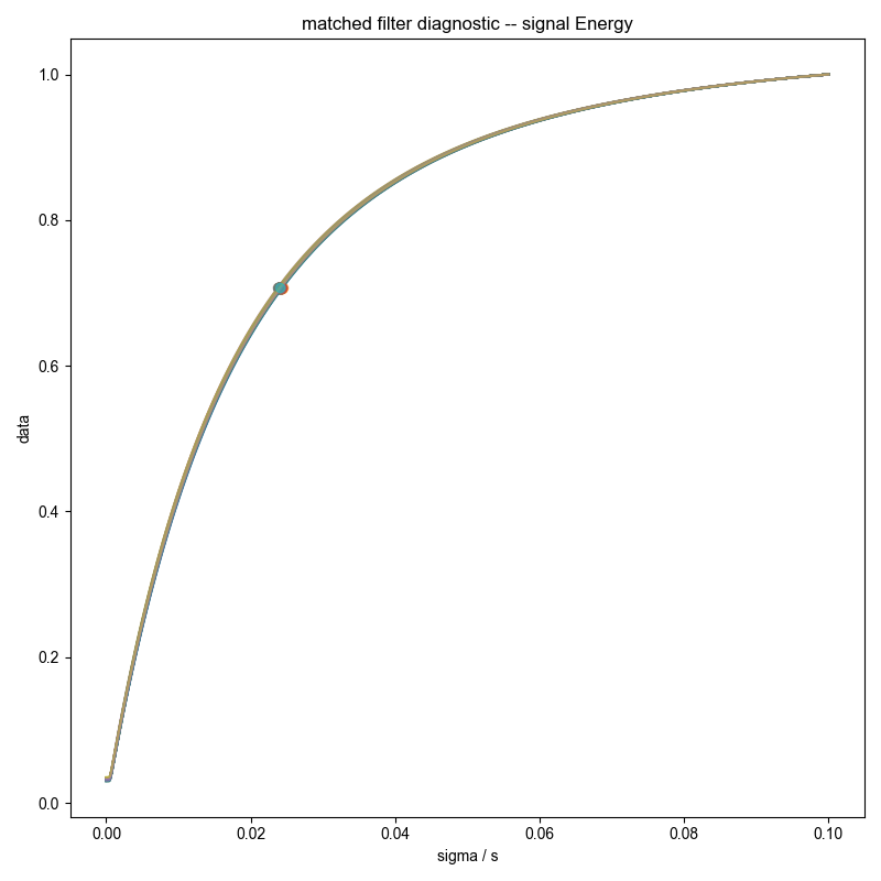
Check integral error calculation

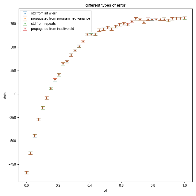
Generate a fake dataset of an inversion recovery with multiple repeats (φ × t2 × vd × repeats) w/ normally distributed random noise. Check that the following match:

• integral w/ error (the canned routine integral_w_errors())

• propagate error based off the programmed σ of the normal distribution

• set the error bars based on the standard deviation (along the repeats dimension) of the real part of the integral

• propagate error based off the variance of the noise in the inactive coherence channels (do this manually inside this script – should mimic what integral_w_errors() does)

• 
• 
• 
• 

----------  logging output to /home/jmfranck/pyspecdata.0.log  ----------
shape of all results [(40, 'vd'), (100, 'repeats')]
#0
#1
#2
#3
#4
#5
#6
#7
#8
#9
#10
#11
#12
#13
#14
#15
#16
#17
#18
#19
#20
#21
#22
#23
#24
#25
#26
#27
#28
#29
#30
#31
#32
#33
#34
#35
#36
#37
#38
#39
#40
#41
#42
#43
#44
#45
#46
#47
#48
#49
#50
#51
#52
#53
#54
#55
#56
#57
#58
#59
#60
#61
#62
#63
#64
#65
#66
#67
#68
#69
#70
#71
#72
#73
#74
#75
#76
#77
#78
#79
#80
#81
#82
#83
#84
#85
#86
#87
#88
#89
#90
#91
#92
#93
#94
#95
#96
#97
#98
#99
off-pathway std array([1.97220022, 1.92375672, 1.97689265, 1.98747806, 1.90421805,
       2.10511932, 2.04874192, 1.97321004, 1.88565543, 2.04797383,
       2.00818674, 2.06696218, 2.02617466, 2.02800179, 1.8381604 ,
       1.9537043 , 2.09145914, 1.98115531, 1.94782724, 1.96258195,
       1.85835747, 1.94830219, 2.03456705, 2.05711269, 2.05529398,
       1.94220362, 1.94225146, 2.09010836, 2.00995428, 2.10428952,
       2.02011849, 1.98634654, 1.9664804 , 1.92916986, 2.00990651,
       2.0238763 , 1.86914168, 1.92370829, 2.02447457, 1.99875205])
        dimlabels=['vd']
        axes={`vd':array([0.        , 0.02564103, 0.05128205, 0.07692308, 0.1025641 ,
       0.12820513, 0.15384615, 0.17948718, 0.20512821, 0.23076923,
       0.25641026, 0.28205128, 0.30769231, 0.33333333, 0.35897436,
       0.38461538, 0.41025641, 0.43589744, 0.46153846, 0.48717949,
       0.51282051, 0.53846154, 0.56410256, 0.58974359, 0.61538462,
       0.64102564, 0.66666667, 0.69230769, 0.71794872, 0.74358974,
       0.76923077, 0.79487179, 0.82051282, 0.84615385, 0.87179487,
       0.8974359 , 0.92307692, 0.94871795, 0.97435897, 1.        ])
                        +/-None}
 programmed std 2.0
/home/jmfranck/git_repos/pyspecdata/pyspecdata/figlist.py:782: UserWarning: Tight layout not applied. The bottom and top margins cannot be made large enough to accommodate all axes decorations.
  plt.gcf().tight_layout()

from numpy import diff, r_, sqrt, real, exp, pi
from pyspecdata import ndshape, nddata, init_logging, figlist_var
from pyspecProcScripts import integral_w_errors

# sphinx_gallery_thumbnail_number = 1

init_logging(level="debug")
fl = figlist_var()
t2 = nddata(r_[0:1:1024j], "t2")
vd = nddata(r_[0:1:40j], "vd")
ph1 = nddata(r_[0, 2] / 4.0, "ph1")
ph2 = nddata(r_[0:4] / 4.0, "ph2")
signal_pathway = {"ph1": 0, "ph2": 1}
excluded_pathways = [(0, 0), (0, 3)]
# this generates fake clean_data w/ a T₂ of 0.2s
# amplitude of 21, just to pick a random amplitude
# offset of 300 Hz, FWHM 10 Hz
clean_data = (
    21 * (1 - 2 * exp(-vd / 0.2)) * exp(+1j * 2 * pi * 100 * t2 - t2 * 10 * pi)
)
clean_data *= exp(signal_pathway["ph1"] * 1j * 2 * pi * ph1)
clean_data *= exp(signal_pathway["ph2"] * 1j * 2 * pi * ph2)
clean_data["t2":0] *= 0.5
fake_data_noise_std = 2.0
clean_data.reorder(["ph1", "ph2", "vd"])
bounds = (0, 200)  # seem reasonable to me
result = 0
n_repeats = 100
all_results = ndshape(clean_data) + (n_repeats, "repeats")
all_results.pop("t2").pop("ph1").pop("ph2")
all_results = all_results.alloc()
all_results.setaxis("vd", clean_data.getaxis("vd"))
print("shape of all results", ndshape(all_results))
for j in range(n_repeats):
    data = clean_data.C
    data.add_noise(fake_data_noise_std)
    # at this point, the fake data has been generated
    data.ft(["ph1", "ph2"])
    # {{{ usually, we don't use a unitary FT -- this makes it unitary
    data /= 0.5 * 0.25  # the dt in the integral for both dims
    data /= sqrt(ndshape(data)["ph1"] * ndshape(data)["ph2"])  # normalization
    # }}}
    dt = diff(data.getaxis("t2")[r_[0, 1]]).item()
    data.ft("t2", shift=True)
    # {{{
    data /= sqrt(ndshape(data)["t2"]) * dt
    error_pathway = (
        set((
            (j, k)
            for j in range(ndshape(data)["ph1"])
            for k in range(ndshape(data)["ph2"])
        ))
        - set(excluded_pathways)
        - set([(signal_pathway["ph1"], signal_pathway["ph2"])])
    )
    error_pathway = [{"ph1": j, "ph2": k} for j, k in error_pathway]
    s_int, frq_slice = integral_w_errors(
        data,
        signal_pathway,
        error_pathway,
        indirect="vd",
        fl=fl,
        return_frq_slice=True,
    )
    # }}}
    manual_bounds = data["ph1", 0]["ph2", 1]["t2":frq_slice]
    N = ndshape(manual_bounds)["t2"]
    df = diff(data.getaxis("t2")[r_[0, 1]]).item()
    manual_bounds.integrate("t2")
    # N terms that have variance given by fake_data_noise_std**2 each
    # multiplied by df
    all_results["repeats", j] = manual_bounds
    print("#%d" % j)
std_off_pathway = (
    data["ph1", 0]["ph2", 0]["t2":bounds]
    .C.run(lambda x: abs(x) ** 2 / 2)  # sqrt2 so variance is variance of real
    .mean_all_but(["t2", "vd"])
    .mean("t2")
    .run(sqrt)
)
print(
    "off-pathway std", std_off_pathway, "programmed std", fake_data_noise_std
)
propagated_variance_from_inactive = N * df**2 * std_off_pathway**2
# removed factor of 2 in following, which shouldn't have been there
propagated_variance = N * df**2 * fake_data_noise_std**2
fl.next("different types of error")
fl.plot(s_int, ".", capsize=6, label="std from int w err", alpha=0.5)
manual_bounds.set_error(sqrt(propagated_variance))
fl.plot(
    manual_bounds,
    ".",
    capsize=6,
    label=r"propagated from programmed variance",
    alpha=0.5,
)
all_results.run(real).mean("repeats", std=True)
# by itself, that would give error bars, but the data would be
# averaged -- better to put the data in the same position
manual_bounds.set_error(all_results.get_error())
# the fact that this matches the previous shows that my sample size is
# large enough to give good statistics
fl.plot(manual_bounds, ".", capsize=6, label=r"std from repeats", alpha=0.5)
manual_bounds.set_error(sqrt(propagated_variance_from_inactive.data))
fl.plot(
    manual_bounds,
    ".",
    capsize=6,
    label=r"propagated from inactive std",
    alpha=0.5,
)
fl.show()